
Calculate how a 5 mm increase in internal pipe diameter affects friction head loss. See Reynolds, Darcy–Weisbach, worked values and charts.
Five millimeters, stated assumptions, and a reproducible calculation
Engineering Laboratory · #01. Five millimeters may look minor when comparing pipes. In hydraulics, internal diameter changes flow area, velocity, and resistance. This first original Andrade Safe study carries 30 liters per minute of water through 20 meters of straight pipe and compares two internal diameters: 20 and 25 mm. Both calculations hold the flow rate fixed.
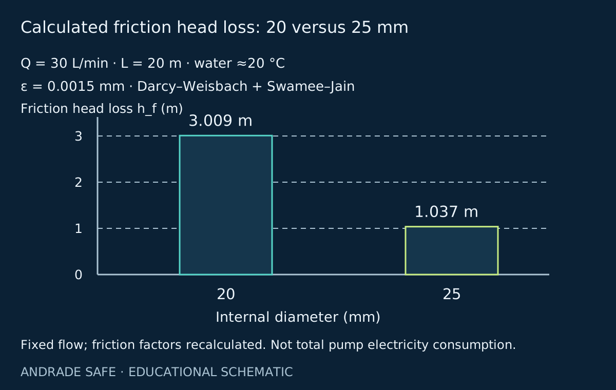
The result is substantial: friction head loss falls from approximately 3.01 to 1.04 meters of water, a reduction of 65.54%. That percentage describes friction in this segment. It does not predict the same percentage reduction in the installation's electricity bill. We will explain the physics, reproduce the calculations, vary the inputs, and put the energy saving in its proper context.
This is a one-dimensional numerical experiment, not a bench measurement or CFD simulation. Calculated charts represent the equations presented; conceptual diagrams explain mechanisms without a design scale. The calculator explores sensitivity, while the table and downloadable files preserve a reproducible analysis when interactive features are unavailable.
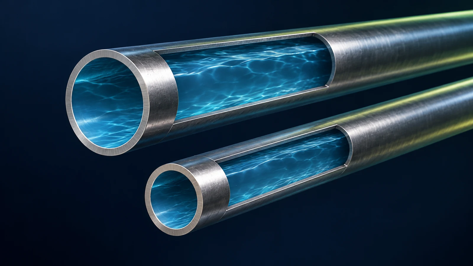
What does head loss mean inside a pipe?
Head loss is the reduction in the flow's mechanical energy per unit weight of fluid. Viscosity and interaction with the wall contribute to dissipation. Energy does not vanish: some mechanical energy becomes internal energy. A pump must provide enough head for the route and the delivery requirements.
Pressure, velocity, and elevation express different energy contributions. In a horizontal, constant-diameter segment with steady flow and no intervening pump, head loss can be related to a pressure drop. If velocity or elevation changes, comparing two pressure gauges without those terms can mislead. Absolute pressure and the pressure difference attributable to friction are also different quantities.
Source: MIT OpenCourseWare — 1.060, Lecture 16: Flow through pipes →
The assumptions held constant
We treat water as liquid, Newtonian, and approximately incompressible at 20 °C. Density is 998.2 kg/m³, dynamic viscosity is 0.001002 Pa·s, and gravitational acceleration is 9.81 m/s². The straight pipe has a circular cross-section and steady flow; the friction model assumes conditions compatible with developed pipe flow. Entrance effects are not resolved in this calculation.
The assumed absolute roughness, 0.0015 mm, represents a very smooth surface. It is not a universal property or a specification for a commercial brand. Length, flow, and fluid properties remain identical; velocity, Reynolds number, and friction factor are recalculated when diameter changes. Fittings and elevation are excluded from the principal result.
For the power attributable to friction, we assume a combined pump–motor efficiency of 60%. Annual operation is 2,000 hours and the illustrative tariff is BRL 0.95/kWh. These are teaching assumptions, not a current electricity quotation or measured efficiency. All appear in the calculator, including adjustable fluid properties under additional options. Currency remains Brazilian reais in every language, without an exchange-rate conversion.
Continuity: equal flow, larger area, lower velocity
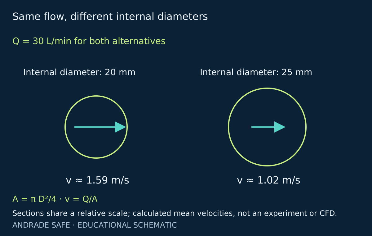
For steady incompressible flow, Q = v · A. A circular area is A = π · D² / 4, giving v = 4Q / (π · D²). Convert 30 L/min to 0.000500 m³/s and enter diameters in meters: 0.020 and 0.025 m. Mixing millimeters and meters at this step changes the result dramatically.
The 20 mm pipe has an area of approximately 0.00031416 m² and mean velocity of 1.59155 m/s. At 25 mm, area becomes 0.00049087 m² and velocity falls to 1.01859 m/s. Diameter increases 25%, area increases 56.25%, and velocity decreases 36.00%. Five millimeters must be understood relative to the original diameter; the same absolute change is not equally significant in every piping system.
Reynolds number and the correct friction factor
Reynolds number compares inertial and viscous effects: Re = ρ · v · D / μ. The values are approximately 31,710 at 20 mm and 25,368 at 25 mm, both clearly turbulent. At fixed flow, increasing diameter reduces velocity and Reynolds number. Friction factor therefore should not automatically be held constant across these alternatives.
We use the Darcy factor, distinct from Fanning: f_Darcy = 4 · f_Fanning. For turbulent flow, the Swamee–Jain approximation is f = 0.25 / [log10(ε / (3.7D) + 5.74 / Re^0.9)]². Roughness ε and diameter D must share units. Calculated factors are 0.023305 for 20 mm and 0.024509 for 25 mm.
The calculator uses f = 64/Re below Re = 2,300 and leaves f and dependent results unavailable from 2,300 to 4,000. These are teaching conventions; actual transition depends on flow conditions. The implementation does not reproduce EPANET's transition interpolation. It flags caution for turbulent calculations near transition and limits ε/D to 0.05 to avoid inappropriate extrapolation in this exercise.
Source: MIT OpenCourseWare — 1.060, Lecture 16: Flow through pipes →
Darcy–Weisbach: the calculation step by step
The equation is h_f = f · (L/D) · v² / (2g). For 20 mm, L/D = 20/0.020 = 1,000 and v²/(2g) ≈ 0.12910 m. Multiplying by f ≈ 0.023305 gives h_f ≈ 3.00879 m. The result has units of length because head represents energy per unit weight.
For 25 mm, L/D = 800, v²/(2g) ≈ 0.05288 m, and f ≈ 0.024509. Head loss is approximately 1.03685 m. Although f increases slightly, the reductions in velocity head and L/D dominate. The difference between the alternatives is approximately 1.97194 meters of water head.
Using Δp_f = ρ · g · h_f converts these losses to 29.463 and 10.153 kPa. They are pressure drops attributable to the friction considered, not absolute delivery pressures. The reduction is (1 − h_f,25 / h_f,20) · 100 = 65.54%. Intermediate calculations retain full precision; rounding is applied only for display.
Source: MIT OpenCourseWare — 1.060, Lecture 16: Flow through pipes →
Diameter sensitivity and an independent cross-check
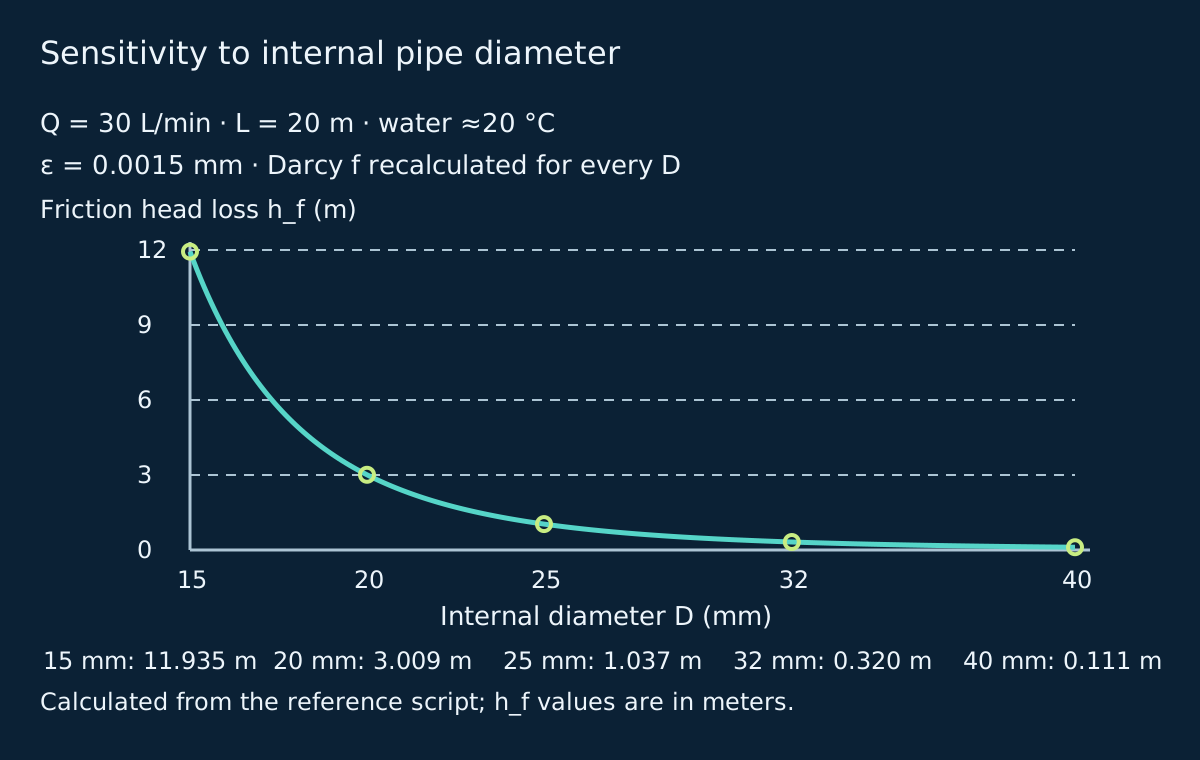
Substituting continuity into Darcy–Weisbach gives h_f = 8 · f · L · Q² / (g · π² · D⁵). With Q, L, and f held constant, loss scales approximately with 1/D⁵. That explains the strong sensitivity, provided the constant-f assumption is stated. In the published calculations, f is recalculated at every diameter.
The table extends the comparison to internal diameters of 15, 20, 25, 32, and 40 mm, all at Q = 30 L/min and L = 20 m. It does not select commercial products. The curve is steep at smaller diameters and falls as diameter grows, without implying that the largest pipe is always the best economic or operational choice.
We also solved Colebrook–White iteratively with identical inputs: 1/√f = −2 · log10[ε/(3.7D) + 2.51/(Re√f)]. The resulting losses are 3.01966 m at 20 mm and 1.04002 m at 25 mm. Swamee–Jain is approximately 0.360% and 0.305% below these values. This agreement checks this particular case; it is not a universal error guarantee for arbitrary inputs.
| Internal D (mm) | v (m/s) | Re | Darcy f | h_f (m) | Δp_f (kPa) | P_e,f (W) | Cost_f (BRL/year) |
|---|---|---|---|---|---|---|---|
| 15 | 2.83 | 42280 | 0.02194 | 11.935 | 116.87 | 97.39 | 185.05 |
| 20 | 1.59 | 31710 | 0.02331 | 3.009 | 29.46 | 24.55 | 46.65 |
| 25 | 1.02 | 25368 | 0.02451 | 1.037 | 10.15 | 8.46 | 16.08 |
| 32 | 0.62 | 19819 | 0.02599 | 0.320 | 3.13 | 2.61 | 4.96 |
| 40 | 0.40 | 15855 | 0.02747 | 0.111 | 1.09 | 0.90 | 1.72 |
Bernoulli with a pump: elevation and fittings still matter
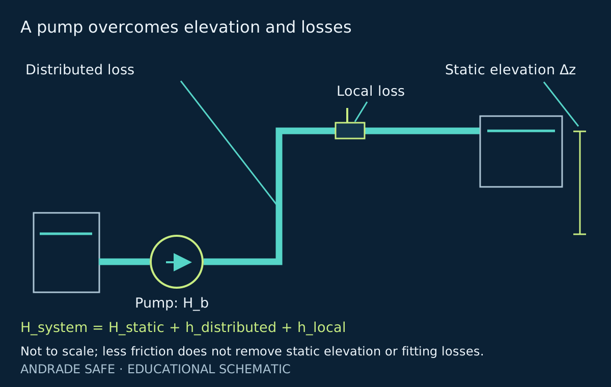
A teaching form of the energy equation between points 1 and 2 is p₁/(ρg) + v₁²/(2g) + z₁ + H_b = p₂/(ρg) + v₂²/(2g) + z₂ + h_losses. The terms describe pressure, velocity, elevation, added pump head, and losses. This simplified form is useful here; a detailed analysis can require kinetic-energy correction factors and the actual endpoint conditions.
System demand combines static head, distributed friction, and local losses. Depending on the selected endpoints, the static contribution also includes the required pressure difference between them. A larger pipe does not remove the elevation water must reach or the pressure required at delivery. The system diagram distinguishes those contributions without supplying dimensions or an executable specification.
Source: MIT OpenCourseWare — 1.060, Lecture 18: Pumping systems →
Power and cost: a large percentage can mean a small monetary saving
Hydraulic power attributable to friction is ρ · g · Q · h_f. Divide by the assumed overall efficiency to obtain P_e,f = ρ · g · Q · h_f / η_overall. With η = 0.60, the results are 24.5526 W and 8.4610 W. This is a theoretical allocation to pipe resistance at fixed flow, not total electrical power measured at the motor.
Multiply by 2,000 annual hours and convert W to kW: energy attributable to friction is 49.1052 versus 16.9219 kWh/year. The difference, 32.1833 kWh/year, is worth BRL 30.57 at the assumed BRL 0.95/kWh. Installation and maintenance costs may show that this small annual saving alone does not justify replacing an existing pipe.
Longer lines, higher flow, or more operating hours can change the scale. Actual savings still require the whole system, controls, and efficiency at the operating point. DOE guidance recommends life-cycle evaluation, including initial investment, energy, and maintenance. An isolated hydraulic percentage does not establish a project's payback period.
Source: Reduce Pumping Costs through Optimum Pipe Sizing — Tip Sheet 9 →
Fixed flow and a fixed-speed pump are different comparisons
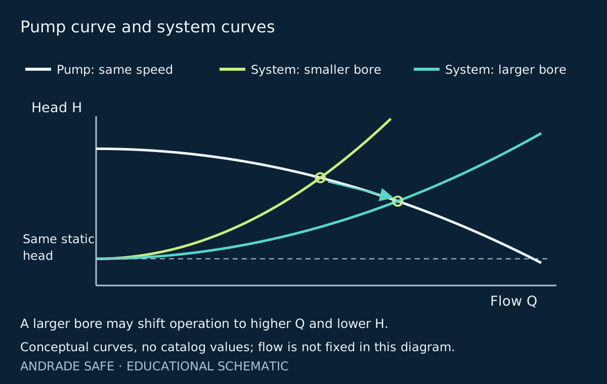
Our experiment sets Q = 30 L/min to isolate diameter sensitivity. In a system with a fixed-speed centrifugal pump, flow follows the interaction of the pump curve and system curve. Their intersection defines an operating point; changing resistance can shift it. In the schematic shown, a larger bore moves the intersection toward higher flow and lower head.
The diagram is conceptual and contains no manufacturer's curve. It cannot predict the new absorbed power, which depends on flow, head, efficiency, and pump and motor characteristics. Control changes, speed adjustment, and throttling also matter. Professional selection requires real curves, suction conditions, and available versus required NPSH with an appropriate margin. The article's calculator does not calculate those quantities.
Source: Improving Pumping System Performance: A Sourcebook for Industry, Second Edition →
Nominal size, roughness, temperature, and local losses
Nominal diameter, outside diameter, and internal diameter are not interchangeable. Wall thickness, SDR, and pressure rating can alter a product's hydraulic area. The example compares 20 and 25 mm internally; commercial specification requires the selected pipe's technical data. Deposits, scale, and aging can change both available bore and surface condition.
Bends, valves, entrances, exits, and connections introduce additional losses, often expressed as h_local = ΣK · v²/(2g). The reference velocity and coefficient must suit each fitting and flow condition. Temperature changes water viscosity; other fluids need appropriate properties. This incompressible model should not be applied directly to compressed air or steam, or treated as the design of a fire protection network.
Try the calculator and reproduce the study
The calculator below adjusts internal diameter, flow, length, roughness, efficiency, annual hours, and tariff. Fluid properties are available under additional options. It updates the selected diameter, the fixed 20 versus 25 mm comparison, and the 15–40 mm curve. When an alternative enters transition, the corresponding loss result becomes unavailable; the curve does not invent an interpolation to fill that gap.
Try doubling length with everything else unchanged: head loss doubles. Then change efficiency alone: head loss and pressure drop stay the same, while allocated electrical power changes. Finally reduce flow and watch Reynolds number. These comparisons separate geometry, flow regime, and energy conversion. Reset restores every assumption in the worked case, not just diameter.
The Python script and supporting spreadsheet in Portuguese reproduce the analysis and are downloadable. Equations and the worked table remain readable without JavaScript. The files are study resources with their stated assumptions and limits. The interactive area does not send entries to third parties or record their values; it does not collect reader data through the calculator.
Try it: friction head loss in a straight pipe
Water at approximately 20 °C. Adjust the inputs: calculations run in this browser without sending your entries.
Fluid properties
Selected diameter results
Flow regime: Turbulent · Swamee–Jain
- Mean velocity (m/s)
- 1.592
- Reynolds number (dimensionless)
- 31,710
- Darcy f (dimensionless)
- 0.02331
- Friction head loss h_f (m)
- 3.009
- Friction pressure drop (kPa)
- 29.46
- Electric power attributable to pipe friction (W)
- 24.55
- Energy attributable to pipe friction (kWh/year)
- 49.11
- Cost attributable to pipe friction (BRL/year)
- 46.65
20 vs 25 mm comparison
Both alternatives use the same flow, length, roughness, and fluid properties. Changing inputs also updates this comparison.
| Internal diameter | h_f (m) | Δp_f (kPa) | P_e,f (W) |
|---|---|---|---|
| 20 mm | 3.009 | 29.46 | 24.55 |
| 25 mm | 1.037 | 10.15 | 8.46 |
Friction head-loss reduction: 65.54%
Internal diameter vs friction head loss — data table
| Internal diameter | h_f (m) | Re |
|---|---|---|
| 15 mm | 11.935 | 42,280 |
| 20 mm | 3.009 | 31,710 |
| 25 mm | 1.037 | 25,368 |
| 30 mm | 0.435 | 21,140 |
| 32 mm | 0.320 | 19,819 |
| 35 mm | 0.209 | 18,120 |
| 40 mm | 0.111 | 15,855 |
This calculator estimates friction loss in an idealized straight pipe; it does not replace system design or pump selection. Power and cost describe only this pipe's friction at fixed flow and efficiency. Elevation, fittings, and the real pump curve are excluded.
What should you take from this first study?
Engineering starts by defining comparable conditions. A geometry change can have a large hydraulic effect, while a practical decision balances investment, operation, and maintenance. A useful calculation states what it includes, what it holds constant, and which decisions still require external information. That discipline applies to a short pipe segment as well as an industrial network.
Possible future studies include pump and system curves, water hammer, vapor-compression cycles and COP, and thermal pipe insulation. These are suggestions for further investigation, without links to unpublished articles or a promised schedule. This edition remains within Mechanical Engineering alongside Andrade Safe's existing content.
Five millimeters are almost invisible to the eye. In a flow equation, they can change the entire discussion.
Explore Mechanical Engineering articles (Portuguese category) →
Frequently asked questions
What is pipe head loss?
Head loss is the reduction in mechanical energy per unit weight caused by dissipative effects, expressed in metres of fluid head. Distributed friction occurs along the pipe; fittings add local losses. Static pressure drop corresponds directly to that loss only when elevation and velocity differences have been properly accounted for.
How do you calculate head loss with Darcy–Weisbach?
Use the internal diameter to calculate area, then v = Q/A and Re = ρvD/μ. Select the Darcy friction factor appropriate to the regime and apply h_f = f(L/D)v²/(2g) with consistent units. Under the published assumptions, the 20 mm pipe loses 3.009 m and the 25 mm pipe 1.037 m at the same 30 L/min flow.
Are pressure drop and head loss the same?
Head loss is dissipated energy per unit weight. Its equivalent pressure is Δp_f = ρgh_f. A measured pressure difference can also reflect elevation and changes in velocity. Static pressure and head loss must therefore be distinguished by applying the energy equation to the measurement points.
Does a larger pipe always reduce electricity use?
At the same flow, length, and conditions, a larger bore tends to reduce friction loss. Actual electricity use depends on pump and system curves, efficiency, and control. With fixed speed, flow can increase. The 65.54% reduction in this exercise describes pipe friction, not a prediction of the electricity bill.
Is DN the internal diameter?
No. DN is a nominal designation and does not necessarily give the hydraulic bore. External diameter, wall thickness, SDR, and pressure class can change a product’s internal diameter. Use the selected pipe’s technical data; this exercise explicitly compares 20 and 25 mm internal diameters.
Which friction-factor formula applies to turbulent flow?
This example uses the Darcy Swamee–Jain expression: f = 0.25/[log10(ε/(3.7D) + 5.74/Re^0.9)]². Colebrook–White was solved as an independent check of this case. The calculator uses 64/Re below 2,300 and gives no friction factor between 2,300 and 4,000; these educational cutoffs do not describe all transition physics.
References
- MIT OpenCourseWare — 1.060, Lecture 16: Flow through pipesMIT OpenCourseWare
- MIT OpenCourseWare — 1.060, Lecture 18: Pumping systemsMIT OpenCourseWare
- EPANET 2.2 User Manual — hydraulic algorithmsU.S. Environmental Protection Agency
- Improving Pumping System Performance: A Sourcebook for Industry, Second EditionU.S. Department of Energy
- Reduce Pumping Costs through Optimum Pipe Sizing — Tip Sheet 9U.S. Department of Energy