
Calculate heat loss from insulated pipes using conduction, convection and radiation. Explore a worked example, graphs and an interactive simulator.
A hot line, a loss that keeps happening
A metal pipe carries water at 90 °C through an industrial area at 25 °C. It looks like a simple run, just 10 meters long. Yet it transfers energy to its surroundings for as long as those conditions persist. How much heat escapes? What changes with 10, 20 or 40 mm of insulation? And why does an additional layer not always reduce heat loss for every possible cylinder? In Engineering 003, we will build a reproducible calculation, follow temperatures through the layers and explore an interactive laboratory. The results apply to explicitly stated teaching assumptions; they are not a promise of savings for every installation.
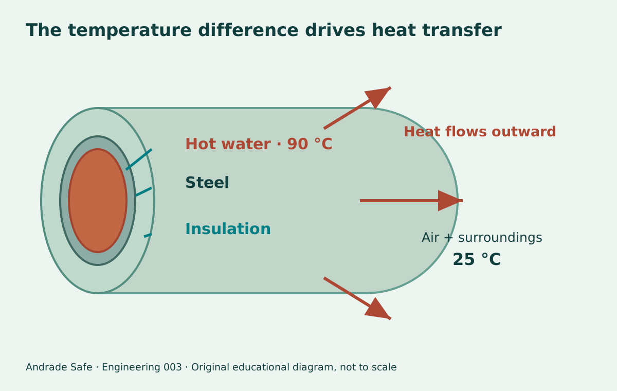
The heat path: water, steel, insulation and surroundings
The temperature difference drives the transfer. First, convection occurs between the water and the inner steel surface. Heat then crosses the metal wall by radial conduction and, when insulation is present, crosses that layer too. At the exposed surface, convection with the air and radiation to the surroundings occur simultaneously. Air does not have to touch the surface for radiative exchange to occur.
The internal stages form a series path: heat has to cross each of them. At the outer boundary, convection and radiation are parallel paths. The surface balance adds their contributions. This arrangement prevents a common mistake: treating radiation as a stage that happens after convection.
Heat-transfer rate Q̇, in watts, measures energy per second. Q̇/L, in W/m, is the heat loss per unit length. Q̇/A, in W/m², is heat-flux density through a particular area. Accumulated energy depends on time and can be expressed in thermal kWh. Because cylindrical area increases with radius, the same heat-transfer rate can cross layers at different heat-flux densities.
Fourier in a cylinder: why does a logarithm appear?
For idealized radial conduction, Q̇ = −k A(r) dT/dr, with A(r) = 2πrL. The minus sign indicates transfer toward lower temperature. Thermal conductivity k has units W/(m·K); radius r and length L are in meters. Under steady conditions, without internal heat generation and with constant k, the heat-transfer rate through every cylindrical surface is the same.
Integrating between two radii gives R_cond = ln(r_outer/r_inner)/(2πkL), in K/W. The radius ratio is dimensionless, and ln is the natural logarithm. This resistance relates the temperature drop across a layer to the transmitted heat-transfer rate. A plane-wall formula with an arbitrarily selected area should not be used when curvature matters.
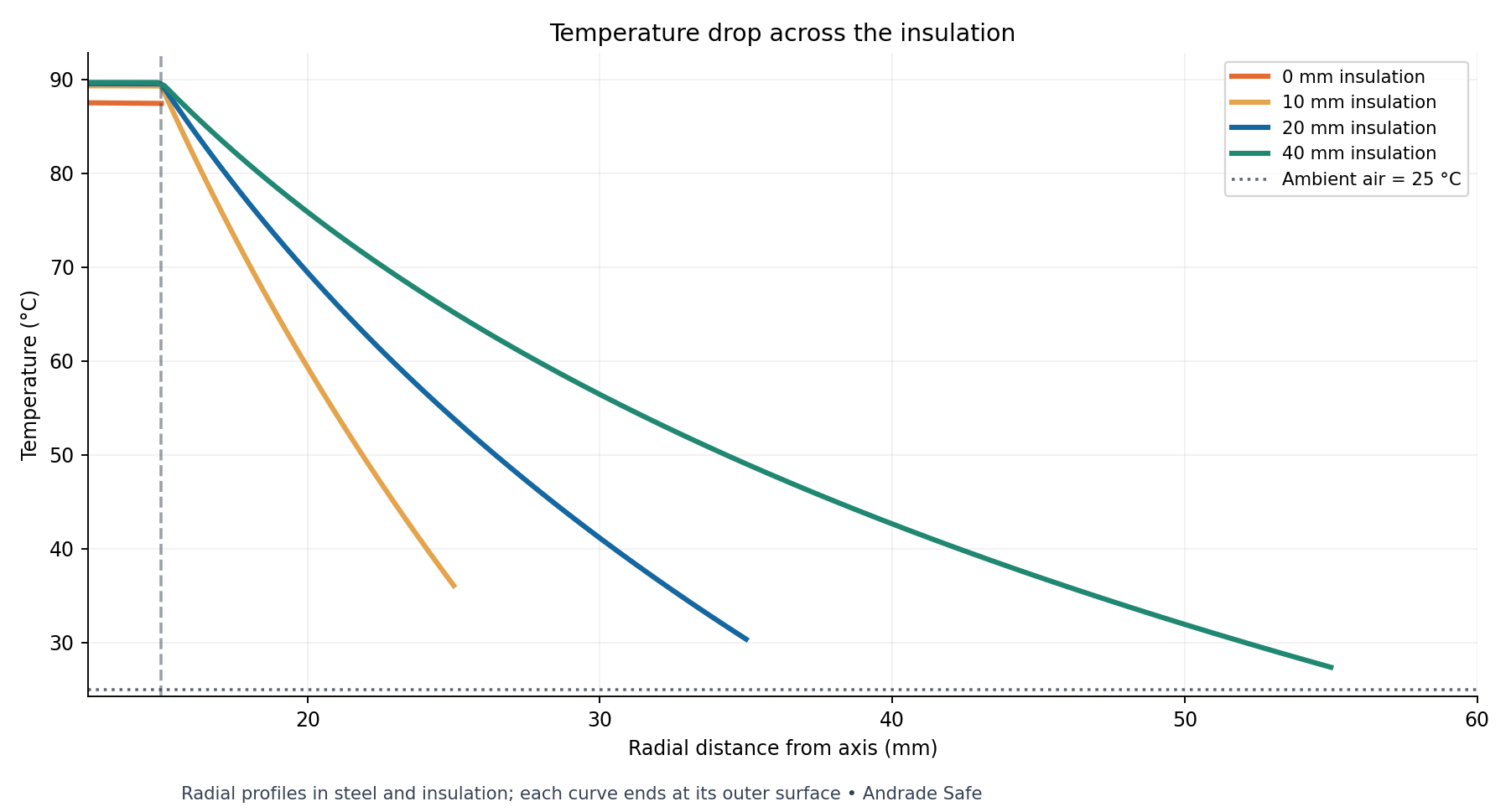
The temperature profile takes the form T(r) = a ln(r) + b within each homogeneous layer. As area increases outward, the magnitude of the gradient decreases with radius for the same heat-transfer rate and conductivity. At a change of material, the slope can change substantially: temperature continuity at an ideal interface does not imply gradient continuity. Contact resistance, when relevant, requires an additional term in the model.
MIT — Heat transfer through a cylindrical wall →
MIT — Combined conduction and convection / critical radius →
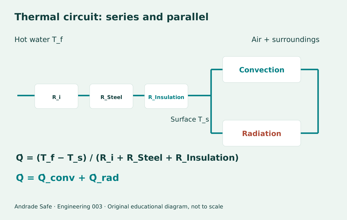
Series resistances, parallel external mechanisms
Let r_i denote the inner steel radius, r_t the outer pipe radius and r_s the outer insulation radius. The internal resistance is R_i = 1/(h_i 2πr_iL). For steel, R_steel = ln(r_t/r_i)/(2πk_steelL). For insulation, R_ins = ln(r_s/r_t)/(2πk_insL). Without insulation, r_s = r_t and R_ins = 0. We define R_int = R_i + R_steel + R_ins.
The rate reaching the surface is Q̇ = (T_f − T_s)/R_int. On the outside, Q̇_conv = h_o A_s (T_s − T_air), with A_s = 2πr_sL. For a small gray surface surrounded by large, uniform radiative surroundings, we use Q̇_rad = εσA_s[(T_s + 273.15)⁴ − (T_surroundings + 273.15)⁴]. The constant σ is 5.670374419 × 10⁻⁸ W/(m²·K⁴).
Radiation requires absolute temperatures in kelvin. In the laboratory, T_surroundings = T_air by assumption; this may be inappropriate in an industrial area near hot equipment. Emissivity ε ranges from zero to one and describes the exposed surface. The calculation uses the same value in every scenario for a controlled comparison, without claiming that bare steel and an actual insulation jacket have equal emissivities.
With radiation disabled, the solution is analytical: Q̇ = (T_f − T_air)/[R_int + 1/(h_o A_s)]. With radiation enabled, the fourth power of temperature makes the balance nonlinear. An equivalent radiative coefficient can be defined from the temperatures, but should not be inserted as a universal constant without justification.
Experiment inputs: what was fixed, and why
The baseline uses a length of 10 m, water at 90 °C, and air and radiative surroundings at 25 °C. The steel radii are 12.5 mm internally and 15.0 mm externally. Insulation thickness is radial: with 20 mm, r_s = 15 + 20 = 35 mm. Do not add the thickness once to the diameter and then use that value as a radius.
We fix properties and coefficients to isolate the effect of geometry. In the field, conductivity may depend on temperature and moisture; convection coefficients depend on flow, orientation and surrounding conditions. Keeping the water uniformly at 90 °C at steady state presupposes heat replenishment or a thermal condition that sustains that state. We do not calculate progressive cooling of the water along the line.
| Parameter | Value |
|---|---|
| L; radii r_i and r_t | 10.0 m; 12.5 mm; 15.0 mm |
| T_f; T_air = T_surroundings | 90 °C; 25 °C |
| k_steel; k_ins | 45; 0.040 W/(m·K) |
| h_i; h_o | 500; 10 W/(m²·K) |
| ε; radiation | 0.80 in all scenarios; enabled |
Worked example: 20 mm of insulation over 10 meters
Step A — convert the geometry: r_i = 0.0125 m, r_t = 0.0150 m and r_s = 0.0350 m. With h_i = 500 W/(m²·K), R_i = 1/(500 × 2π × 0.0125 × 10) ≈ 0.002546 K/W. For steel, R_steel = ln(0.015/0.0125)/(2π × 45 × 10) ≈ 0.0000645 K/W.
Step B — calculate the insulation resistance: R_ins = ln(0.035/0.015)/(2π × 0.040 × 10) ≈ 0.33713 K/W. Insulation resistance dominates this internal sum; that does not remove the need to represent external exchange. The surface area is A_s = 2π × 0.035 × 10 ≈ 2.1991 m².
Step C — find T_s so that incoming heat equals outgoing heat. The balance function is F(T_s) = (90 − T_s)/R_int − Q̇_conv(T_s) − Q̇_rad(T_s). At 25 °C, external outflow is zero and F is positive; at 90 °C, inflow through the wall is zero and F is negative. A root exists between these temperatures. At the first bisection trial, T_s = 57.5 °C: outflow exceeds inflow, so the next search is between 25 and 57.5 °C. Repeatedly divide the interval until convergence.
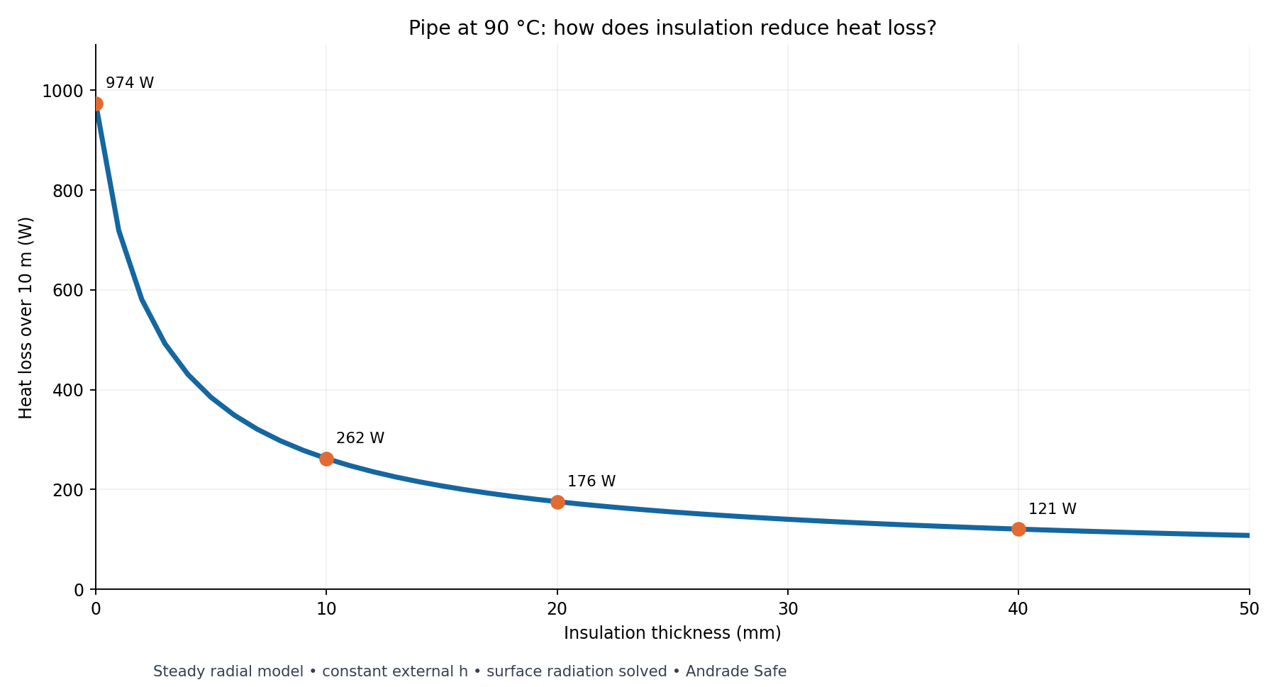
Step D — the numerical result is T_s ≈ 30.34 °C and Q̇ ≈ 175.59 W, or 17.56 W/m. Convection carries approximately 117.53 W and radiation 58.06 W. Their sum closes the surface balance. Python, the spreadsheet and the article engine calculate this same condition; differences in displayed values arise only from rounding.
| Insulation | Total Q̇ (W) | Q̇/L (W/m) | T_s (°C) | Reduction vs. bare pipe |
|---|---|---|---|---|
| 0 mm | 973.76 | 97.38 | 87.46 | 0.0% |
| 10 mm | 262.02 | 26.20 | 36.06 | 73.1% |
| 20 mm | 175.59 | 17.56 | 30.34 | 82.0% |
| 40 mm | 120.58 | 12.06 | 27.35 | 87.6% |
Radial profile and sensitivity: what insulation actually changes
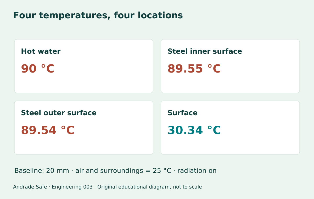
With 20 mm, the water remains at 90 °C, the inner steel surface is approximately 89.55 °C and its outer surface is 89.54 °C. The insulation surface is at 30.34 °C, while the air is at 25 °C. These are distinct temperatures. The largest drop through the solid layers occurs in the insulation because its resistance is much higher, not because the steel has stopped conducting heat.
The radial-profile chart shows logarithmic segments and ends at the surface of each scenario. It does not show the temperature distribution in the air or inside the water. The transition from surface temperature to ambient temperature is represented by a boundary condition, not by extending the conduction curve through the air.
Ignoring radiation affects the uninsulated reference most strongly: the prediction falls from 973.76 W to 597.90 W. With 20 mm, it changes from 175.59 W to 168.74 W. The insulated surface is closer to ambient temperature, reducing the absolute radiative effect. Do not calculate a reduction using a bare pipe without radiation and compare it with an insulated pipe with radiation: both references must follow the same model.
| Thickness | Convection only | Convection + radiation |
|---|---|---|
| 0 mm | 597.90 | 973.76 |
| 20 mm | 168.74 | 175.59 |
Interactive laboratory: experiment with insulation
Change thickness, temperatures, external convection, conductivity, length, emissivity and radiation. The chart and results use the same balance solved by bisection. Steel radii, steel conductivity and internal convection remain fixed and are shown alongside the controls. The field ranges define this teaching experiment; they are not universal limits for materials or equipment.
The uninsulated reference is recalculated using the same selected parameters. Hours, price and efficiency govern only the economic estimate. If these fields are missing or invalid, the thermal calculation remains available, but cost results are not displayed. The tool models a hot line: enter a fluid temperature higher than ambient temperature. Do not automatically convert a cold-line case into a condensation analysis.
Lab: heat loss from a pipe
Change the inputs. Calculations run in your browser without sending your values.
Steady radial model. Steel radii: 12.5 and 15 mm; h_i = 500 W/(m²·K); k_steel = 45 W/(m·K). T_surroundings = T_air; properties and emissivity fixed within each comparison. Wind, axial cooling, supports, flanges, moisture, contact resistance and material selection are not calculated.
- Total heat loss Q̇ (W)
- 175.59
- Linear heat loss (W/m)
- 17.56
- Surface temperature (°C)
- 30.34
- Reduction versus bare pipe (%)
- 82.0
- Thermal energy lost (kWh/year)
- 702.37
- Replacement cost (BRL/year)
- 619.74
- Hypothetical gross savings (BRL/year)
- 2,817.08
- External convection (W)
- 117.53
- External radiation (W)
- 58.06
Calculated scenario table
| Thickness (mm) | Q̇ (W) | T_s (°C) |
|---|---|---|
| 0 | 973.76 | 87.46 |
| 10 | 262.02 | 36.06 |
| 20 | 175.59 | 30.34 |
| 30 | 140.24 | 28.33 |
| 40 | 120.58 | 27.35 |
| 50 | 107.88 | 26.78 |
| 60 | 98.89 | 26.41 |
Theoretical critical radius k/h: 4.00 mm. Only for the convection-only model, without radiation, at constant k and h. This is total outer radius, not added thickness; not an exact limit for the radiation model.
(T_f − T_s)/R_int = h_o A_s (T_s − T_air) + εσA_s (T_s,K⁴ − T_air,K⁴). Bisection solution; the second term is zero when radiation is off.
Amounts in Brazilian reais (BRL), using an assumed input energy price and full replacement of heat loss at the stated efficiency. Not a promised electricity-bill reduction or a payback calculation.
Critical radius: why can more insulation increase heat loss from a thin wire?
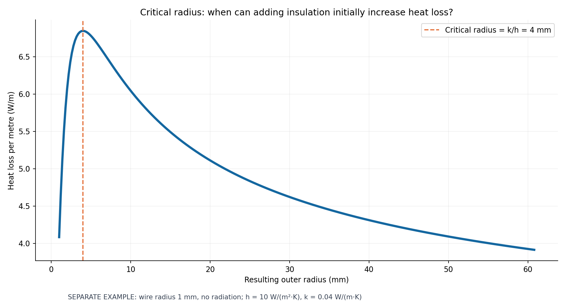
For a cylinder with constant external convection and no radiation, an additional layer increases conduction resistance but also increases external area. The larger area reduces convection resistance. This competition yields the critical radius r_crit = k_ins/h_o. For k_ins = 0.040 W/(m·K) and h_o = 10 W/(m²·K), r_crit = 0.004 m = 4 mm.
This is the total outer radius of the assembly, not insulation thickness. Our pipe already has an outer radius of 15 mm, greater than 4 mm. Therefore, in this simplified convection model, adding insulation reduces its loss from the outset. The baseline chart with radiation also shows a reduction, calculated from its own balance; we do not use k/h to claim an exact limit for that radiation model.
The small example in the chart below is a different system: a wire of radius 1 mm, with an interface prescribed at 90 °C, air at 25 °C, no radiation and none of the internal resistances of the main pipe. Loss starts at approximately 4.084 W/m, rises to approximately 6.846 W/m at an outer radius of 4 mm, and then falls. The peak corresponds to a 3 mm added layer. This distinction makes the counterintuitive phenomenon physically understandable.
MIT — Combined conduction and convection / critical radius →
From watts lost to annual savings: a conditional calculation
Thermal energy lost at a constant rate is E_thermal = (Q̇/1000) × hours, in kWh/year. To estimate purchased energy used to replace this loss, divide by heat-generation efficiency η. Cost is C = (Q̇/1000) × hours × price/η. Price refers to input energy, and efficiency describes its conversion into useful heat in this scenario; it is not the COP from the previous article.
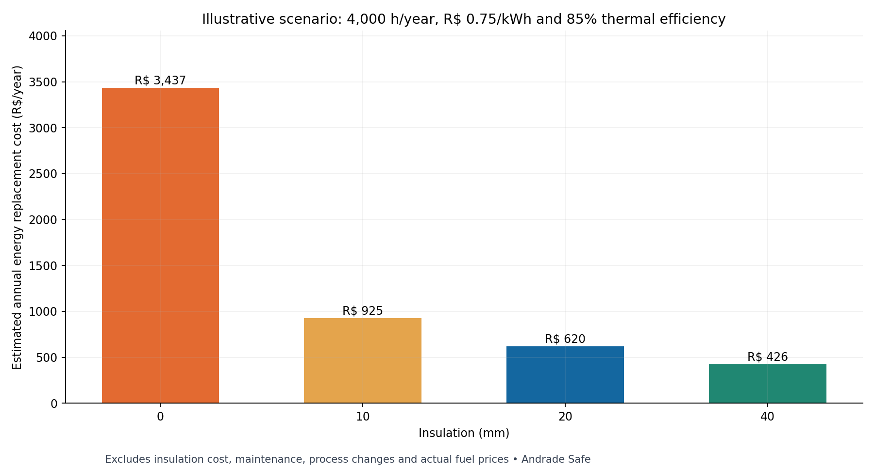
Using 4,000 h/year, BRL 0.75/kWh of input energy and η = 0.85, the estimated bare-pipe cost is BRL 3,436.81/year. With 20 mm, it is BRL 619.74/year. The difference, BRL 2,817.07/year, is hypothetical gross savings in heat replenishment. The 82% reduction in heat loss belongs to the example, not a guarantee of an installation’s electricity-bill reduction.
The benefit depends on whether lost heat actually needs replacing, how it is generated and what other losses exist. DOE treats insulation as an opportunity in steam systems, but its examples and percentages are not our results for water at 90 °C. We do not calculate payback without installed investment, maintenance, service life and operating conditions. Marginal savings from additional thickness must also be compared with its additional cost.
U.S. Department of Energy — Insulate Steam Distribution and Condensate Return Lines →
U.S. Department of Energy — Improving Steam System Performance: A Sourcebook for Industry →
| Condition | Cost (BRL/year) |
|---|---|
| Bare pipe | 3,436.81 |
| 10 mm | 924.79 |
| 20 mm | 619.74 |
| 40 mm | 425.59 |
Surface temperature: a useful result for safety
The predicted surface temperature falls from 87.46 °C on the bare pipe to 30.34 °C with 20 mm under the laboratory assumptions. This indicates a relevant change in exposure to hot surfaces and thermal exchange with the occupied area. But one calculated value does not authorize declaring the whole installation safe to touch.
Burn risk depends on actual temperature, surface material and finish, contact duration and skin conditions. Flanges, supports, joints and uninsulated sections may remain hot even when the modeled run’s surface is cooler. Professional assessment must examine the assembly, its operation and the applicable technical criteria.
Insulation also needs integrity: moisture protection, finishing, continuity and provision for inspection. Damaged or wet insulation may perform differently from a calculation with constant k. Predicted temperature is information for design and verification, not an automatic protection certificate.
Where the model ends — and real design begins
The laboratory is radial and steady-state. It does not calculate startup, shutdown or energy storage in the layers. It does not include thermal bridges at supports, flanges and valves, or water-temperature decline along long lines. Such situations may require combining an axial fluid balance with local radial transfer and changes over time.
Also outside the model are insulation moisture and compaction, variable k, contact resistance, additional layers and radiative exchange with equipment at different temperatures. External h is an input, not a prediction from wind speed or natural-convection correlations. Internal h is constant and is not recalculated from flow rate.
A cold line receives heat from the surroundings, but condensation analysis requires humidity, dew point, a vapor barrier and appropriate properties. Steam lines may need treatment of phase change and their own operating conditions. Tools such as 3E Plus help with insulation assessments; our laboratory does not reproduce their methods or replace manufacturer data and design verification.
Calculation workbook: download and reproduce
The workbook brings together a spreadsheet, Python model, CSV, HTML simulator and complete kit. Calculation files are in Portuguese; all three article versions have text, captions, tables and laboratory content adapted to their language. The kit charts preserve the supplied data and composition, with a revised radial-profile title.
The spreadsheet contains inputs and formulas; Python uses the standard library to solve the balance and produce CSV, with optional matplotlib for generating charts. The HTML can be opened locally in a browser with JavaScript. For publication, we corrected preservation of the chart’s accessible title and description, and a spreadsheet label that stated “10 m” even though length was editable. We also revised the radial-profile title to “Temperature drop across the insulation” in the localized chart. The model and baseline values were preserved.
Use the declared ranges and assumptions. The spreadsheet does not apply all the field validations used by the blog laboratory; physically invalid values may produce meaningless results. Recalculation was checked in the spreadsheet engine available in this session; behavior in native Excel and browser review have not been verified.
Insulation is a decision about where energy should flow
Adding insulation changes thermal resistance, external area, surface temperature and replenishment cost. Doubling thickness does not mean halving loss: 20 mm and 40 mm produce approximately 175.59 W and 120.58 W in this case. A benefit exists, but it does not follow a universal linear rule.
The engineering series connects three questions: how much it costs to move water through a pipe, how electrical work transports heat, and how much heat a line loses to its surroundings. In each, decisions improve when we define the boundary, check units and keep assumptions visible.
Insulating a pipe means applying engineering to a temperature difference: understanding the heat path, calculating how much escapes, and deciding in context how much it is worth reducing that loss. This laboratory’s most valuable benefit is learning to build that interpretation and recognize when a more complete model is needed.
Frequently asked questions
How do you calculate heat loss from an insulated pipe?
Add internal convection resistance and radial conduction resistances through the layers. At the surface, balance that heat-transfer rate against the sum of convection and radiation. Without radiation, the model has an analytical solution; with radiation, surface temperature is solved numerically. Radii, coefficients, properties and boundary conditions must be consistent.
Does twice as much insulation halve the loss?
Not necessarily. Cylindrical resistance depends on the logarithm of the radius ratio, while external area also changes. In the baseline, increasing thickness from 20 to 40 mm reduces loss from 175.59 to 120.58 W over 10 meters. This is a comparison within this model, not a universal rule.
Why is the temperature profile logarithmic?
In steady radial conduction with constant conductivity and no internal generation, the same heat-transfer rate crosses areas that increase with radius. Integrating Fourier’s law in this geometry produces a logarithmic function. The profile applies within each layer and does not automatically describe the water or outside air.
What is the critical radius of insulation?
It is the outer radius that maximizes loss in a purely convective cylindrical model with constant h and k. The expression is r_crit = k/h. It is not the added thickness. With variable radiation, this expression should not be applied as an exact result without reviewing the boundary condition.
Can insulation increase heat loss?
It can happen initially in a very thin cylinder when the increase in external area outweighs added conduction resistance. The small wire example, with a radius of 1 mm, shows this behavior without radiation. The main pipe has a radius of 15 mm, beyond the 4 mm critical radius of the convection example.
Must radiation calculations use kelvin?
Yes: the fourth power must use absolute temperature. The laboratory converts °C to K by adding 273.15. Temperature differences in convection and conduction have the same numerical value in °C and K, but raising degrees Celsius to the fourth power in the radiation equation gives an incorrect calculation.
Do thermal savings equal a lower electricity bill?
Not automatically. The replenishment calculation considers hours, input-energy cost and heat-generation efficiency, assuming the loss needs replacing. The installation may use other energy sources and have additional losses. BRL 2,817.07/year for 20 mm applies only to the stated hypothetical scenario.
Is a surface at 30 °C automatically safe?
Safety of the whole installation should not be certified from a predicted temperature. Actual conditions, material, contact duration, exposed parts and applicable criteria must be checked. The model indicates reduced temperature in an idealized run; it does not assess every location or exposure mode.
Does the simulator calculate wind or select the appropriate material?
No. It takes external h and insulation k as constant inputs and keeps steel geometry and internal convection fixed. It does not select a product or evaluate moisture or installed cost. The charts show the effect of entered parameters within the laboratory ranges.
Does the model apply to cold pipes and condensation?
The laboratory is defined for fluid hotter than the surroundings. Cold lines require a separate analysis of heat gain, humidity, dew point and vapor barriers. Simply reversing the loss sign is not enough to interpret the result as a condensation check.
References
- Heat transfer through a cylindrical wallMIT
- Combined conduction and convection / critical radiusMIT
- Insulate Steam Distribution and Condensate Return LinesU.S. Department of Energy
- Improving Steam System Performance: A Sourcebook for IndustryU.S. Department of Energy
- 3E PlusNAIMA / Insulation Institute
- Process heat and steamAustralian Government