
Understand machine vibration and resonance: natural frequency, damping, amplitude calculations, FFT and equipment diagnostics.
The machine vibrates: what question should we ask?
The motor turns, the pump operates and the assembly begins to vibrate. This may seem an inevitable consequence of rotation. But a periodic force can excite a structural mode and produce motion much greater than its static response. To understand this difference, we need to follow natural frequency, damping and excitation conditions.
Vibration is not necessarily the fault. Machines and structures respond to varying forces because they have mass, elasticity and dissipation mechanisms. Diagnosis starts with frequency, amplitude, direction, phase and trend, related to operation. Not all high vibration is resonance; resonance alone does not establish that failure will occur.
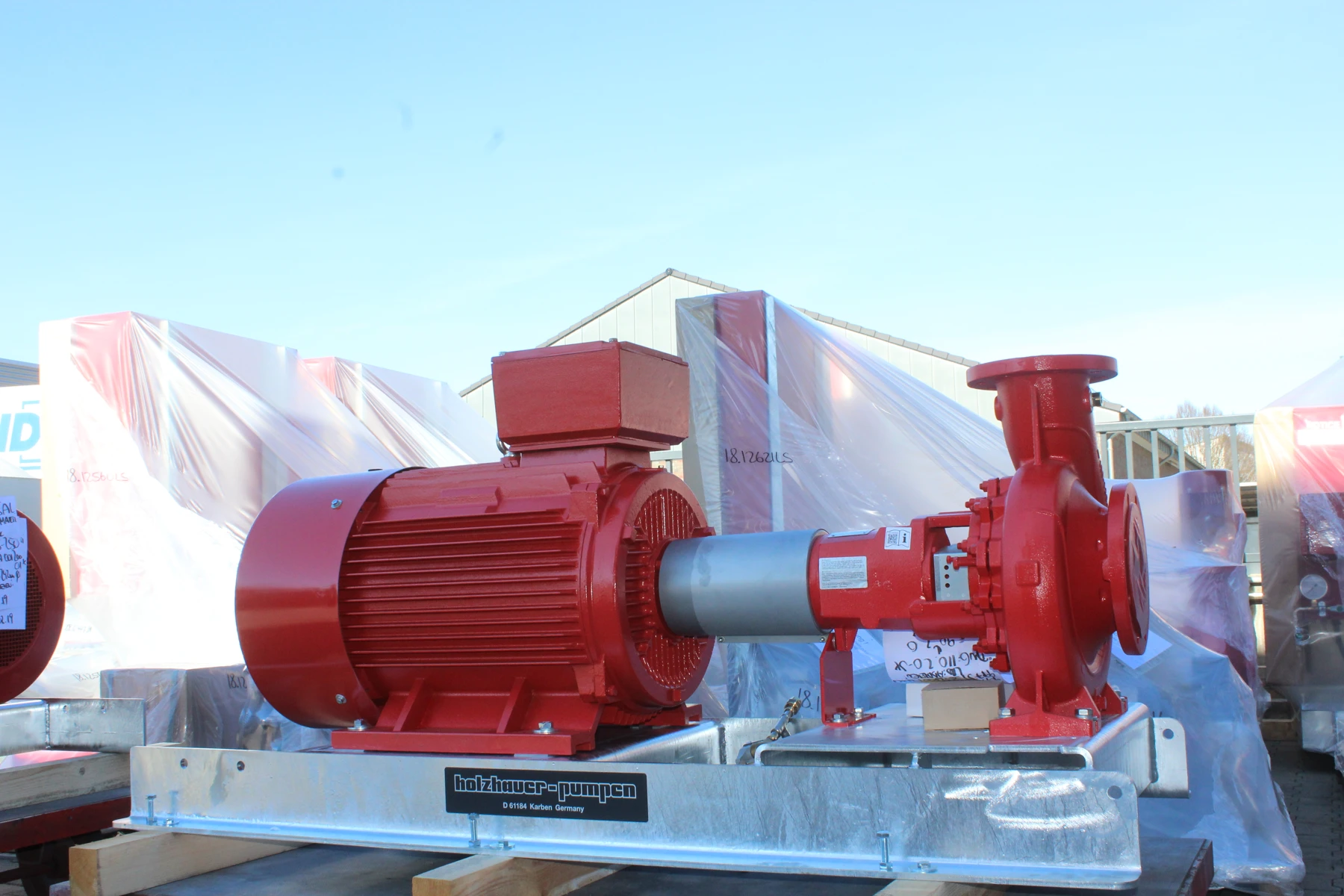
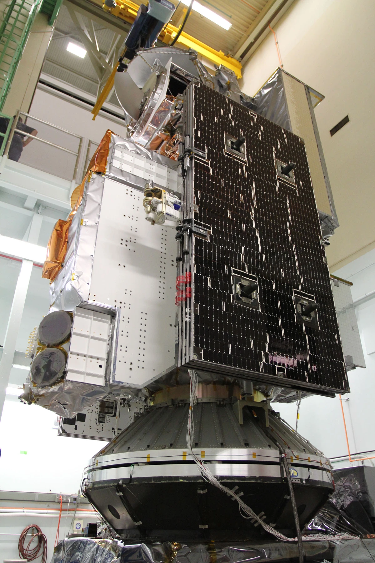
This edition connects the pump and fatigue articles through a narrative review of university materials and public standards summaries. Calculations and the spectrum are synthetic. Photographs show equipment and tests identified in the credits; they depict neither the exercise’s machine nor measurements performed by Andrade Safe.

Four layers of knowledge, four purposes
MIT OpenCourseWare materials support the study of free vibration, forced response and systems with multiple degrees of freedom. Public summaries of ISO 13373-1 and 20816-1 provide context for collection and evaluation. Instrumentation documentation helps interpret acquisition and spectra. These sources answer complementary questions and are not interchangeable.
This is a narrative review of the materials consulted, without a systematic search, meta-analysis or bibliometric survey. We do not claim full consultation of paid standards or cite pages of books that were not examined. The example equations are applied to declared assumptions rather than presented as experimental results.
A model describes mechanisms; sensors measure responses; relevant criteria guide comparison; diagnosis links signals to testable hypotheses. Confusing these layers can turn a calculated amplitude into a standards-based classification unsupported by the data.
| Layer | Question | Limit |
|---|---|---|
| Linear vibration | How do mass, stiffness and damping control response? | An SDOF does not describe every mode |
| Modal analysis | Which frequencies, damping ratios and mode shapes exist? | They depend on configuration and supports |
| Monitoring | Where, how and under what conditions should measurements be taken? | An isolated sample does not necessarily identify the cause |
| Evaluation | Which trend and criteria apply? | No universal mm/s RMS limit applies to every machine |
Mass, spring and damper: the SDOF model
The single-degree-of-freedom, or SDOF, model uses one coordinate x to represent a dominant motion. For an external harmonic force, mẍ + cẋ + kx = F₀ sin(ωt). Effective modal mass m is in kg; stiffness k in N/m; viscous damping c in N·s/m; x in m; F₀ in N; and ω in rad/s.
Undamped natural frequency is ω_n = √(k/m), or f_n = ω_n/(2π). The damping ratio is ζ = c/(2√(km)); the frequency ratio is r = ω/ω_n = f/f_n. These are distinct quantities: f_n belongs to the system and f to excitation. Rotation may generate excitation related to f but does not automatically define natural frequency.
A real machine has multiple motions and couplings. SDOF is useful for understanding an approximate dominant mode, not for locating cracks or independently reconstructing the entire installation. Changes in mass, stiffness and supports may change frequencies; temperature, load and configuration must also be considered.

Free vibration: what happens after an impulse?
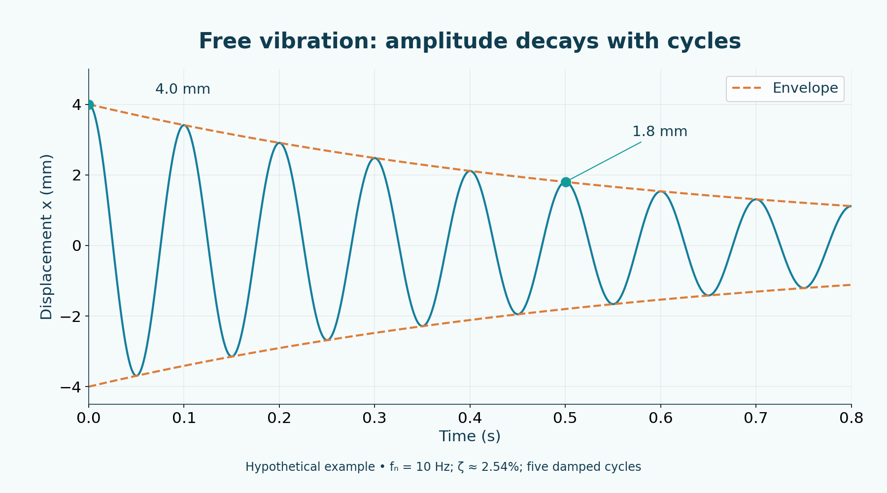
Without a continuous external force, an underdamped system can oscillate after initial conditions. For 0 < ζ < 1, damped frequency is ω_d = ω_n√(1 − ζ²), and the envelope decays proportionally to exp(−ζω_nt). The frequency observed during decay is not exactly the undamped natural frequency.
Peaks of the same sign separated by n cycles allow estimation of δ = ln(x_i/x_(i+n))/n. Then ζ = δ/√(4π² + δ²). This assumes a dominant mode and decay consistent with the linear model; simply choosing two peaks from a signal containing impacts and multiple superimposed frequencies is insufficient.
In the example, 4.0 mm and 1.8 mm five cycles later give δ = ln(4/1.8)/5 = 0.15970154 and ζ = 0.02540908, or 2.54%. This identification exercise is independent of the 4% assembly used later. Shaker-table photographs document real tests, but the free-vibration curve remains an educational construction.
| Item | Value |
|---|---|
| Same-sign peaks | 4.0 mm and 1.8 mm |
| Separation | 5 cycles |
| δ | 0.15970154 |
| ζ | 0.02540908 = 2.54% |
Forced response: amplification and phase lag
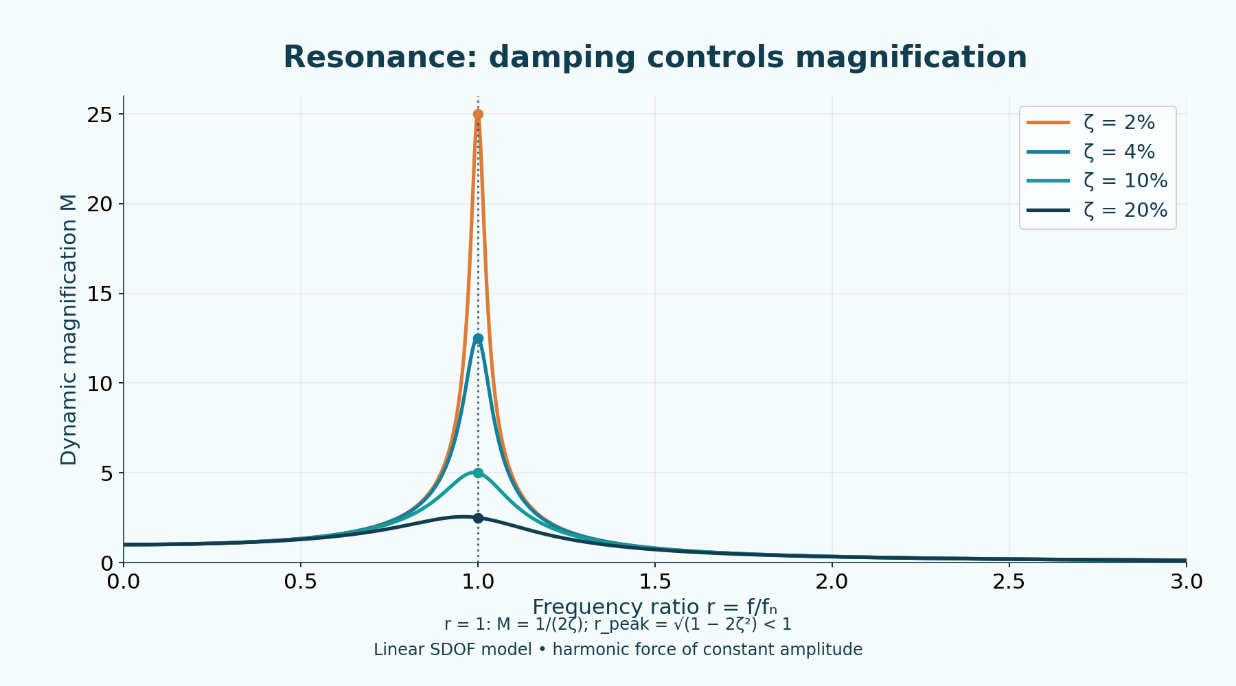
With a sinusoidal force of constant amplitude at steady state, X = (F₀/k)/√[(1 − r²)² + (2ζr)²]. X is peak displacement; F₀/k is the static deflection under the same force. Amplification M = X/(F₀/k) is dimensionless. It is neither a stress measurement nor an acceptable-vibration limit.
At r = 1, M = 1/(2ζ). With ζ = 4%, response is 12.5 times static deflection. The exact displacement peak for constant force occurs at r_p = √(1 − 2ζ²) when 0 < ζ < 1/√2, slightly below one. This condition should not be applied indiscriminately to other excitation types or metrics.
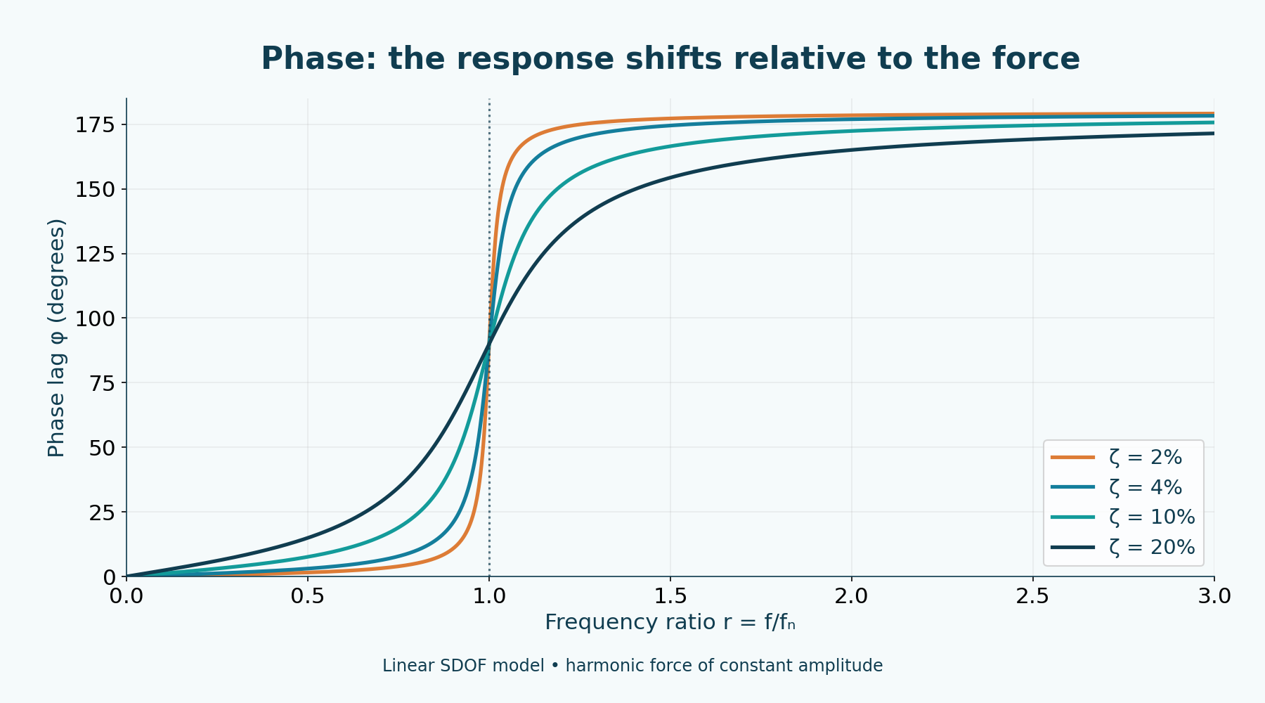
Phase lag can be written φ = atan2(2ζr, 1 − r²). At f = f_n, it is 90°. Using atan2 preserves the quadrant as frequency crosses the natural-frequency region. At steady state, x(t) = X sin(ωt − φ); this curve does not include the startup transient.
With low damping, a coarse frequency grid may miss the narrow peak. The lab includes natural frequency, the analytical peak and the selected point, with local refinement. This correction improves mathematical representation; real measurement still requires appropriate acquisition and interpretation.
Exercise: a hypothetical assembly with a mode at 30 Hz
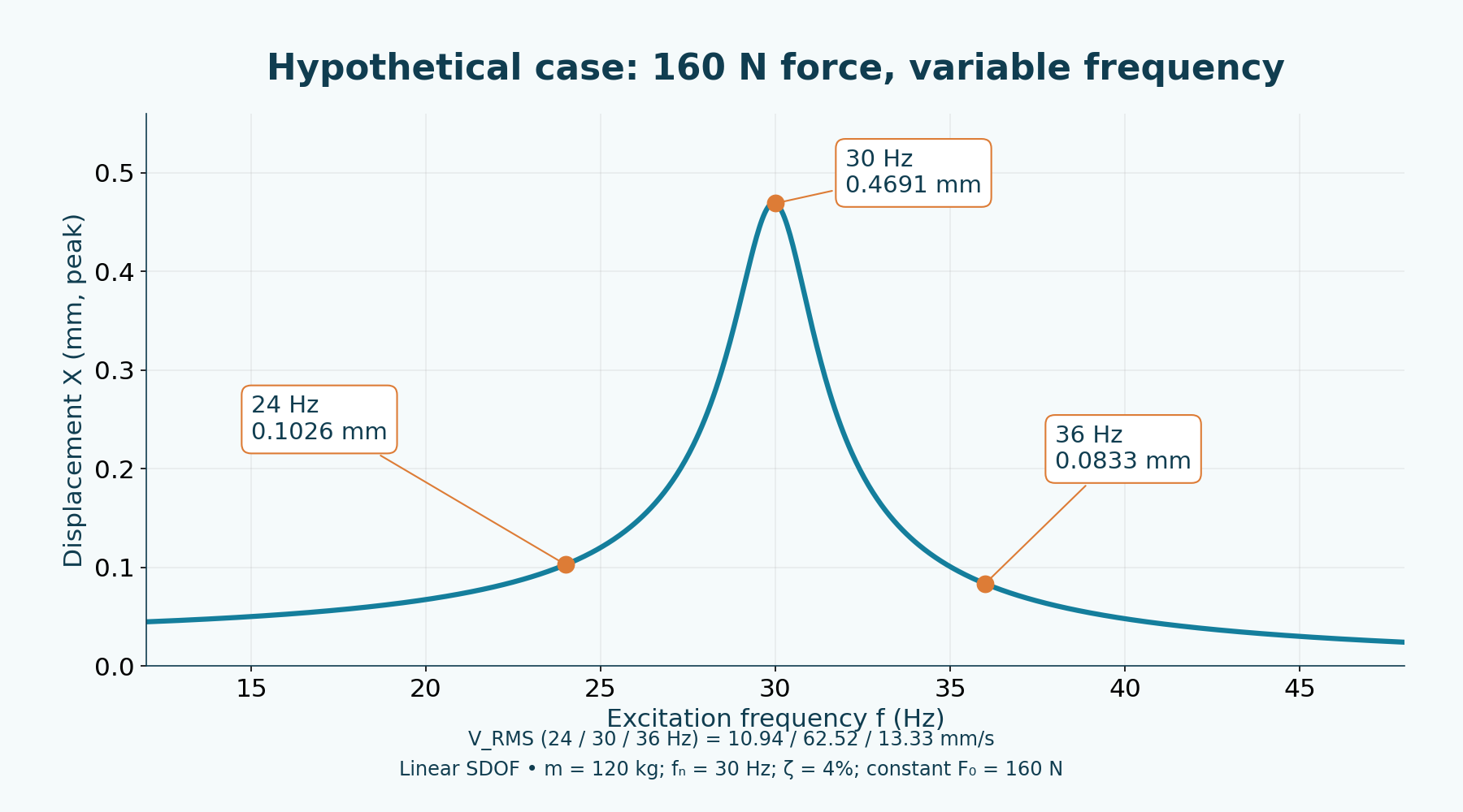
We adopt a modal mass of 120 kg, f_n = 30 Hz, ζ = 4% and a constant peak harmonic force F₀ = 160 N. Equivalent stiffness is k = 120(2π×30)² = 4263669.101 N/m, approximately 4.264 MN/m. Static deflection is 160/k = 0.03752636 mm.
At 30 Hz, r = 1 and M = 12.5. Peak displacement is X = 0.46907955 mm. Peak velocity is ωX ≈ 88.42 mm/s; for this sinusoid, V_RMS = ωX/√2 = 62.521966 mm/s. Peak acceleration is ω²X = 16.666667 m/s². Peak and RMS should not be mixed.
The high velocity belongs to the fictional scenario. It was not measured on the photographed pump and receives no generic ISO classification. Assumptions of linearity, fixed force amplitude and one dominant mode make the comparison transparent but may cease to represent a real assembly under certain conditions.
| f | M | Peak X | Sinusoidal V_RMS | Peak acceleration |
|---|---|---|---|---|
| 24 Hz | 2.734896 | 0.102631 mm | 10.943428 mm/s | 2.333778 m/s² |
| 30 Hz | 12.500000 | 0.469080 mm | 62.521966 mm/s | 16.666667 m/s² |
| 36 Hz | 2.220490 | 0.083327 mm | 13.327625 mm/s | 4.263342 m/s² |
Rotational frequency is not synonymous with natural frequency
A speed of 1800 rpm corresponds to 30 Hz. The equivalence f = rpm/60 identifies first-order excitation, 1×, when present. Other components may relate to blade passing, gear meshing or electrical forces. An induction motor may also run at an actual speed different from nominal because of load and slip.
In the exercise, F₀ remains constant when f changes. This matters: an imbalance force may grow approximately with ω² under usual assumptions. The educational amplification curve therefore does not independently predict a machine’s response across its entire speed range. The operational spectrum combines sources with structural response.
With f = 30 Hz, increasing ζ from 4% to 12% reduces X to 0.156360 mm and V_RMS to 20.840655 mm/s in the model. Keeping mass, force, 4% damping and f = 30 Hz, changing f_n to 38 Hz gives X = 0.061230 mm and V_RMS = 8.161075 mm/s. These are sensitivity studies, not implementation-ready corrections to an installation.
What should change: source, structure, dissipation or operating regime?
Reducing excitation may involve addressing causes of imbalance, misalignment or looseness after diagnosis. Changing stiffness, mass or fastening may shift modes; increasing stiffness does not necessarily move every natural frequency away from operation. The outcome depends on the system’s starting condition and which modes matter.
Damping may reduce peaks, but materials and devices must be evaluated within the assembly. Speed ranges, starts, stops and variable-frequency drives may also pass through critical regions. An intervention must be verified under comparable conditions, considering other responses and components.
No single formula authorizes balancing, reinforcing or installing isolators on every machine. Decisions require distinguishing the excitation source from structural response and considering function, limits, integrity and operating conditions. A reduction in one overall number alone does not prove the cause has been resolved.
Isolation: force transmissibility to the support
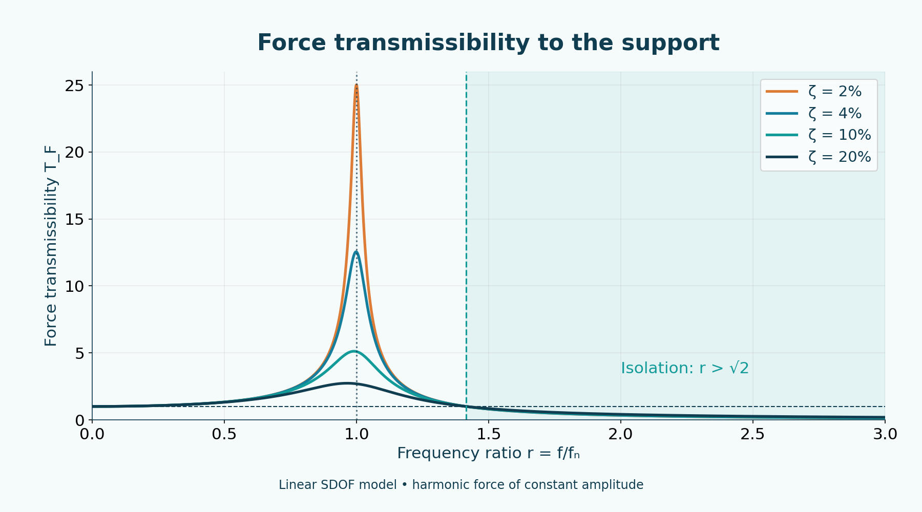
For a harmonic force applied to the SDOF mass, the ratio of force amplitude transmitted to the support to excitation-force amplitude is T_F = √[1 + (2ζr)²]/√[(1 − r²)² + (2ζr)²]. It is not simply machine displacement. Comparing transmissibility requires identifying the input and output being related.
In this model, T_F < 1 when r > √2. This shows why an isolator can amplify response near resonance before reaching the isolation region. Greater damping helps in the resonance region but may increase transmissibility at high frequency ratios.
Real selection considers supported mass, stability, permissible deflections, transients, environment and connections. Hoses, pipes and other links may also create transmission paths. The expression does not size an isolator or replace assessment of the assembly’s modes.
Measurement: displacement, velocity and acceleration
The procedure must characterize equipment, process condition, load, speed, temperature, locations and directions. ISO 13373-1 addresses vibration monitoring and general procedures, including acquisition and sensor aspects. Comparison is meaningful only when configuration and operating state are sufficiently known.
Displacement in µm or mm may be relevant to larger motions and low frequencies, or relative shaft measurements where appropriate. RMS velocity in mm/s is used in overall assessment of certain machine types. Acceleration in m/s² or g may help observe higher-frequency components and impacts. Bandwidth, sensor, mounting and conditioning change the result’s meaning.
The relationship RMS = peak/√2 applies to a sinusoid. A real signal containing impacts or multiple components may have a different crest factor. Integration and differentiation also require instrumentation care; not every acceleration record can be converted into reliable velocity without examining acquisition, bandwidth and processing.
FFT: separating frequencies does not automatically reveal the cause
The FFT is an algorithm for the discrete Fourier transform. It reveals the frequency content of a sampled record, subject to duration, window, noise and acquisition. Nyquist frequency is f_s/2; antialias filtering and a practical margin are needed to prevent out-of-band components from being interpreted as other frequencies.
Bin spacing is Δf = f_s/N = 1/T for the original samples. The effective ability to separate tones also depends on the window and signal-to-noise ratio. A window may reduce spectral leakage but changes amplitude and lobe width; it does not eliminate every problem. Zero-padding interpolates the spectrum without creating additional physical information.
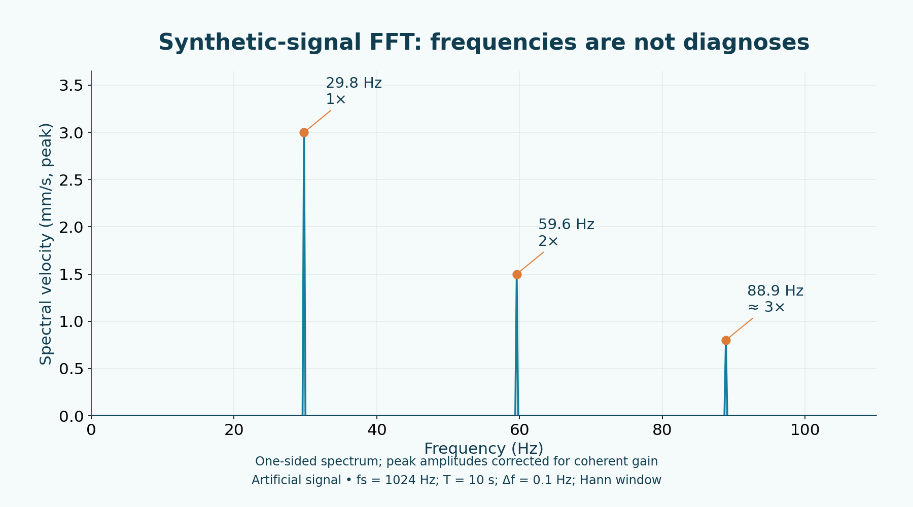
In the artificial example, the reference is 29.8 Hz, equivalent to 1788 rpm. The signal contains 29.8 Hz, 59.6 Hz and 88.9 Hz. The third component is near 3×, not exact: 3×29.8 = 89.4 Hz. A 1× peak alone does not prove imbalance; 2× alone does not prove misalignment. Phase, directions, trend and independent evidence remain necessary.
The chart was generated with f_s = 1024 Hz, a 10 s record, N = 10240 and a Hann window. The axis shows one-sided peak amplitude in mm/s, with coherent-gain correction; Δf = 0.1 Hz. It is neither overall RMS velocity measured in a factory nor a diagnosis of the photographed equipment.
FFT and modal analysis answer different questions
An operating spectrum simultaneously contains excitations and structural response. Modal analysis seeks to estimate natural frequencies, damping and mode shapes. In a conventional experimental test, force and response are measured to form frequency response functions, FRFs, using appropriate instruments and procedures.
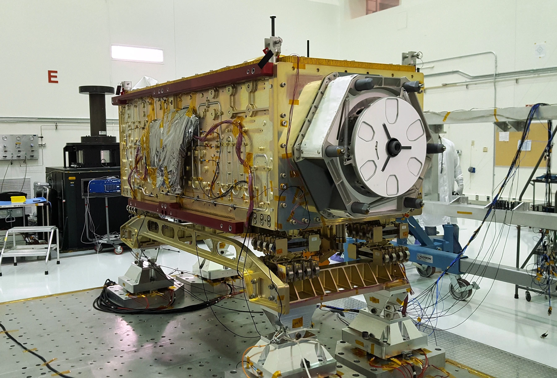
Instrumented hammers, exciters and sensors may take part in these tests. Photographs of NASA/JPL and NASA Goddard tests show real vibration-testing contexts without representing measurements from our example. A vibration qualification test should not automatically be called modal identification merely because a shaker table is present.
Real systems have multiple degrees of freedom, bending and torsional motions, supports and couplings. SDOF teaches the phenomenon’s grammar; a real machine requires understanding many coexisting modes and forces. Neither an isolated FFT nor this lab replaces modal testing, a structural model or evidence-based diagnosis.
MIT — Lecture 24, multiple degrees of freedom →
ISO 20816: criteria depend on the machine and applicable part
At the editorial check, ISO 20816-1:2016 remained published, while the second edition was under publication at stage 60.00. A field indicating October 2026 was not treated as confirmation that the edition had already been published. ISO 13373-1:2002 also remained published, with confirmation in September 2024.
Metadata and public summaries were consulted. ISO 20816-1 provides general measurement and evaluation guidelines; limits and conditions must be associated with the relevant part and equipment. There is no single mm/s RMS value that universally classifies motors, pumps, fans and every structure.
Assessing a level requires identifying quantity, bandwidth, location, support, operating condition and applicable criteria, as well as trend. The calculated 62.52 mm/s RMS belongs to the hypothetical sinusoid and is not automatically transferred into a standards-based evaluation zone.
ISO 20816-1:2016 — public scope and status →
Connecting fatigue to a traceable field study
High dynamic response can increase cyclic stresses depending on mode and geometry. However, overall displacement does not directly give local stress in a weld or bolt. A structural model, strain measurement or justified modal relationship is needed. Vibration, resonance and fatigue are related but distinct phenomena.
The fatigue edition explains stress amplitude and mean, concentration, cycles and crack growth. Resonance can worsen a load history but does not independently establish life or rupture. Traceable conditions and evidence allow the link between measured response and integrity to be built.
In the field, a study must start from known conditions, safe access and acquisition documentation. Intervention is followed by a new comparable measurement, without declaring the problem solved merely because one isolated value decreased.
Metal fatigue: stress, cycles and cracks →
- Characterize equipment, function, history, load and speed.
- Define access and a measurement procedure compatible with the hazards.
- Document sensor, location, direction, mounting, bandwidth and settings.
- Collect a baseline under known, repeatable operating conditions.
- Compare trends, spectra, phase and independent evidence.
- Justify intervention and measure again under comparable conditions.
Lab: compare frequency, damping and response
Change modal mass, natural frequency, damping, peak force and excitation frequency. The lab calculates stiffness, ratio r, amplification, peak displacement, sinusoidal RMS velocity, peak acceleration, phase and force transmissibility. Equivalent tables let you read results without relying solely on charts.
Keep f_n = 30 Hz, ζ = 4% and F₀ = 160 N to compare 24, 30 and 36 Hz. Then try ζ = 12% at 30 Hz and f_n = 38 Hz with excitation fixed at 30 Hz. When mass changes while f_n remains fixed, the lab recalculates k proportionally: this does not represent adding mass while retaining the same spring.
The time series contains five periods of steady-state harmonic response without a startup transient. Calculations run locally in the browser; they are not sensor data or ISO limits. Trilingual HTML, Python, CSV and a package with figures and credits are available. Without JavaScript, consult the static exercises; controls do not update results.
Vibration and resonance laboratory
Change five parameters and compare the steady-state sinusoidal response.
Linear single-degree-of-freedom model with constant peak force. It does not classify machines or approve a design.
- Stiffness k (N/m)
- 4,263,669.10127
- Frequency ratio r
- 1
- Amplification M
- 12.5
- Peak displacement (mm)
- 0.46908
- RMS velocity (mm/s)
- 62.52197
- Peak acceleration (m/s²)
- 16.66667
- Phase (degrees)
- 90
- Force transmissibility
- 12.53994
View equivalent chart data
| f (Hz) | M | X (mm) | V RMS (mm/s) | A (m/s²) |
|---|---|---|---|---|
| 24 | 2.7349 | 0.10263 | 10.94343 | 2.33378 |
| 29.95196 | 12.51001 | 0.46946 | 62.47185 | 16.62664 |
| 30 | 12.5 | 0.46908 | 62.52197 | 16.66667 |
| 36 | 2.22049 | 0.08333 | 13.32762 | 4.26334 |
| t (s) | x (mm) |
|---|---|
| 0 | -0.46908 |
| 0.02083 | 0.33169 |
| 0.04167 | -0 |
| 0.0625 | -0.33169 |
| 0.08333 | 0.46908 |
| 0.10417 | -0.33169 |
| 0.125 | 0 |
| 0.14583 | 0.33169 |
| 0.16667 | -0.46908 |
k=m(2πf_n)²; M=1/√[(1−r²)²+(2ζr)²]; X=F₀M/k; V_RMS=2πfX/√2
ζ = 0.04 means 4%. Changing m at fixed f_n recalculates k; it does not add mass to the same spring. RMS = peak/√2 applies here to a sinusoid. Force does not increase with speed in this model.
Open the standalone PT/EN/ES lab →
Calculating, measuring and interpreting belong to the same decision
Natural frequency and damping explain why a force can produce different responses depending on its frequency. Measurement adds the machine’s reality: sources, supports, modes, process and history. Diagnosis requires relating these elements without turning a simple model into certainty about equipment.
Resonance is not an engineering superstition. It is a predictable physical response. The professional challenge is not just calculating when it may occur but measuring, interpreting and deciding correctly what to do when it does.
Frequently asked questions
What is natural frequency?
It is a dynamic characteristic associated with a system’s mass, stiffness and conditions. In an undamped SDOF, f_n = √(k/m)/(2π). A real machine may have multiple frequencies and mode shapes affected by supports, load, temperature and configuration. Natural frequency is not automatically equal to rotational frequency or a peak observed in operation; identifying a mode requires context and appropriate analysis.
Does resonance always cause failure?
No. It is a dynamic amplification condition whose response depends on excitation, damping, modes and system limits. It can increase motion and stress, but failure requires assessing actual mechanisms and conditions. Nor should all intense vibration be assumed to be resonance. Models and measurements help formulate and verify hypotheses without making a peak automatic proof of damage.
How do you calculate natural frequency?
For a single-degree-of-freedom mass and spring, use ω_n = √(k/m) and f_n = ω_n/(2π), with m in kg and k in N/m. This calculation represents the adopted model. In real structures with multiple degrees of freedom, frequencies and mode shapes depend on mass and stiffness distribution and constraints and may require modeling and testing. Total mass and an assumed stiffness alone are insufficient.
What does vibration in mm/s RMS mean?
It is an effective measure of vibration velocity within a defined bandwidth and condition. For a single sinusoid, RMS equals peak divided by √2; real signals may have a different crest factor. Interpretation requires knowing sensor, mounting, direction, processing and operation. The 62.52 mm/s example is calculated rather than measured and receives no universal standards classification.
What is the difference between FFT and modal analysis?
FFT reveals components of a sampled record, which may combine excitation and response. Modal analysis seeks natural frequencies, damping and mode shapes using appropriate procedures and relationships; a conventional test measures force and response to form FRFs. An isolated operating spectrum does not automatically identify modes. Window, sampling, duration and test conditions also affect conclusions.
Does a 1× peak prove imbalance?
No. 1× corresponds to the frequency associated with reference rotational speed, but multiple sources and responses can produce content at that order. Imbalance is a hypothesis that must be checked against phase, direction, trend, support conditions and other evidence. Likewise, 2× alone does not prove misalignment. The article’s synthetic spectrum is for studying frequencies, not diagnosing a machine.
How can vibration be reduced?
Response may change through reduced excitation, changes in mass or stiffness, damping, isolation and operating regime. Selection depends on diagnosis and assembly assessment. Reinforcing a base does not necessarily move every mode away from operation; isolators may also amplify near resonance. After intervention, compare measurements under known conditions and examine more than a single overall number.
Does ISO 20816 provide one limit for every machine?
No. Part 1 provides general guidelines, and assessment must identify the applicable part, machine, measured quantity, bandwidth and relevant conditions. This edition consulted public summaries and standards status without the full paid text. We do not use the lab’s value as an ISO limit or classify the photographed installations as approved or rejected.
Can vibration cause fatigue?
It can contribute to cyclic stresses depending on structure, mode and loading. Fatigue also depends on stress amplitude and mean, cycles, concentrations, material and environment. No universal direct conversion exists from overall displacement to local joint stress. The relationship requires a model, strain measurement or a justified modal transfer; resonance, vibration and fatigue are not identical phenomena.
References
- MIT — Engineering Dynamics: Mechanical VibrationMIT OpenCourseWare
- MIT — Lecture 21, Thomas Peacock, 7 May 2007MIT OpenCourseWare
- MIT — Problem Set 9, Engineering DynamicsMIT OpenCourseWare
- MIT — Lecture 24, multiple degrees of freedomMIT OpenCourseWare
- NI — Understanding FFTs and WindowingNI
- NI — FFT FrequencyNI
- NI — Bandwidth and Nyquist samplingNI
- Brüel & Kjær — Structural testing, BR0507Brüel & Kjær
- SKF — Vibration spectrum analysisSKF
- ISO 20816-1:2016 — public scope and statusISO
- ISO 20816-1 — Edition 2, under publicationISO
- ISO 13373-1:2002 — public scope and statusISO
- pump-photo.webpReal centrifugal pump and motor assembly, used only to illustrate rotating machinery; it is not the equipment in the worked example. Photo: HopuWiki / Wikimedia Commons, CC BY-SA 4.0. Resized and converted to WebP.
- oco-testing-photo.webpOCO-3 on the vibration table in the JPL environmental test laboratory, with cables connected to test sensors. Courtesy NASA/JPL-Caltech, PIA23211. Historical photograph from 2019, resized and converted to WebP.
- gpm-testing-photo.webpGPM spacecraft attached to the shaker table for horizontal vibration testing at Goddard. Photo: Warren Shultzaberger / NASA, 2013. Resized and converted to WebP.