
Understand centrifugal pumps, learn to read H–Q curves, find the operating point and assess NPSH and cavitation.
If the motor is turning, why is the water not arriving?
A pump is switched on, its motor is turning, yet the installation still has insufficient flow. The problem may lie in selection, circuit resistance, suction or operating conditions that differ from those anticipated. Electrical current and shaft movement alone do not demonstrate that the assembly delivers the required hydraulic energy.
The central idea is simple: a pump does not determine flow on its own. The operating point arises from the meeting between what the machine offers and what the installation demands. To understand that interaction, we will follow the fluid through the impeller, read two curves, solve an example and examine the physical limit represented by NPSH.
The photographs show real equipment identified in the sources and credits. The curves and numbers are hypothetical: they do not belong to those pumps or represent an approved selection. The simulator lets you explore this model without accessing installations or sending values to external systems.

How does a centrifugal pump transfer energy to fluid?
Liquid reaches the impeller eye near the shaft and receives energy from the rotating blades. Flow is directed toward the periphery; the casing or a diffuser collects the fluid and allows part of its kinetic energy to be converted into pressure. The pump supplies energy per unit weight of liquid, expressed as head H.
Head is not simply a building’s physical height. Added energy appears in the pressure, velocity and elevation balance between reference points. For the same H, the corresponding pressure difference depends on density. In this study we use water with ρ = 1000 kg/m³; the meters shown are meters of liquid.
A conventional centrifugal pump may depend on priming and appropriate suction conditions to work as intended. An assembly with air in the flow path, incorrect rotation or incompatible resistance may fail to achieve expected performance. These are diagnostic hypotheses, not instructions for intervening in energized equipment.
Impeller, volute, seal and motor: what does each do?
The impeller transfers energy; the casing contains the fluid and organizes its discharge; the suction nozzle guides liquid to the inlet, and the discharge nozzle delivers it to the circuit. In the diagram of a horizontal end-suction pump, the inlet aligns with the shaft and the discharge appears on the casing. Other constructions have different geometries.
The shaft transmits torque from the drive to the impeller. Bearings support rotation, while the sealing system limits fluid passage around the shaft. Mechanical seals and other arrangements have their own compatibility and operating requirements. The motor converts electrical energy into mechanical energy, with losses distinct from the pump’s hydraulic losses.
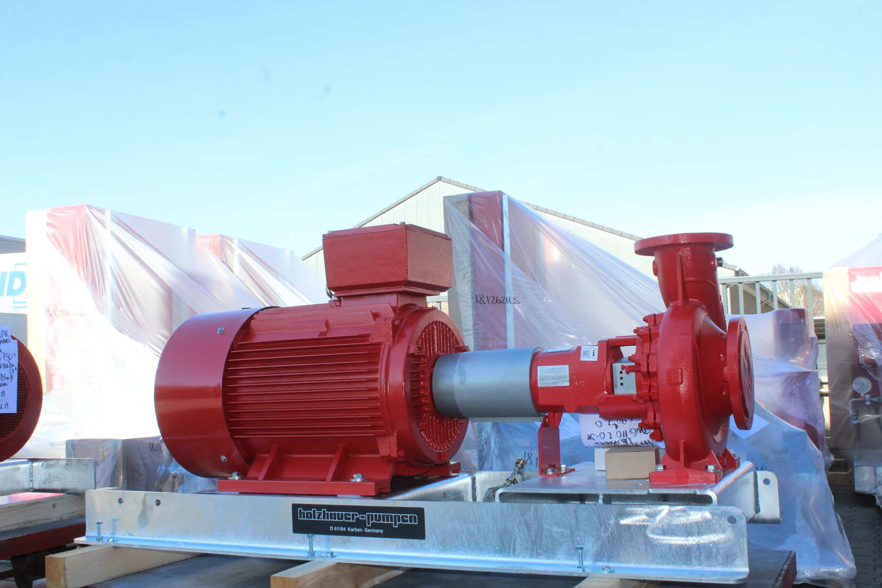
The photograph of a complete assembly helps distinguish pump from motor; the educational section view helps trace fluid inside the casing. None of these images alone provides a machine’s performance curve, operating range or required NPSH.

The H–Q curve: the energy the pump offers
A pump curve relates flow Q and head H for specified speed, impeller and fluid conditions. In many centrifugal pumps, head decreases as flow increases. This does not make every real curve a universal parabola: different families and regions behave differently, and manufacturer data guides selection.
For teaching, we adopt H_p(Q) = 45 − 0.05 Q², with H in m and Q in m³/h. The 45 m is the model’s shutoff head at zero flow. The coefficient has units of m/(m³/h)². If Q is converted to m³/s, the same numerical coefficient cannot be retained without converting the expression.
The curve is shown only within the nonnegative-head domain. It reaches H = 0 at Q = √(45/0.05) = 30 m³/h; we do not extend the expression to portray a machine delivering negative head or a zero-head plateau. Nor do we use shutoff as a recommended condition for continuous operation.
The system curve: what the installation demands
The installation requires energy to overcome differences in elevation and pressure as well as losses in pipes, fittings, valves and equipment. We represent this demand as H_s(Q) = 8 + 0.02 Q². In this example, 8 m is the static component, and the quadratic term approximates losses that increase with flow.
This static component may include pressure between reservoirs; it should not always be confused with elevation difference. In a closed HVAC circuit returning to the same point, geometric elevation is not automatically the net static head to overcome on every circuit. Circuit losses remain, and pressurization also matters for suction.
The kQ² term is an educational approximation. In real hydraulic calculations, length, diameter, roughness, fittings, flow regime and fluid properties determine losses. The friction factor may vary with Reynolds number; reducing everything to constant k is useful for comparing scenarios but does not size a network.
Worked example: where do the curves meet?
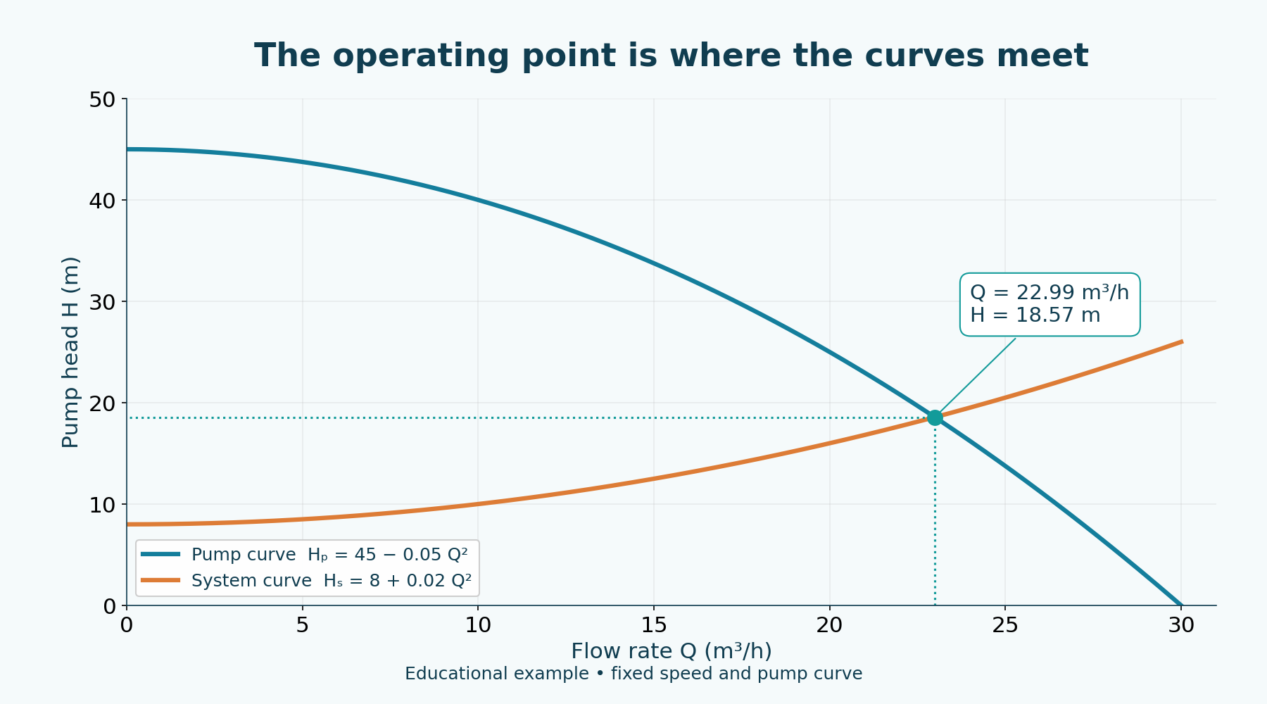
The model’s operating point satisfies H_p = H_s: 45 − 0.05 Q² = 8 + 0.02 Q². Rearranging gives 37 = 0.07 Q²; therefore Q = √(37/0.07) = 22.990681 m³/h. We choose the positive root, consistent with the adopted flow direction.
Substituting the unrounded flow, H = 45 − 0.05 × 528.571429 = 18.571429 m. The system curve, 8 + 0.02 × 528.571429, gives the same result. The final presentation is approximately 23.0 m³/h and 18.6 m. The chart shows the intersection, but the equality lets us check the value.
For H_p = H₀ − aQ² and H_s = H_static + kQ², the solution is Q = √[(H₀ − H_static)/(a + k)] within this study’s domain. If H₀ ≤ H_static, no positive flow is predicted. The simulator flags this condition rather than inventing a point at Q = 0 with mismatched curves or calculating shaft power from it.
Hydraulic Institute — Combined Pump and System Curves →
| Item | Value |
|---|---|
| Pump curve | H_p = 45 − 0.05 Q² |
| System curve | H_s = 8 + 0.02 Q² |
| Q² | 528.571429 (m³/h)² |
| Q | 22.990681 m³/h |
| Converted Q | 0.006386300 m³/s |
| Head H | 18.571429 m |
| Condition | Mathematical intersection; not catalog selection |
Hydraulic, shaft and electrical power: three quantities
Power delivered to the liquid is P_h = ρ g Q H. Here Q must be entered in m³/s: 22.990681/3600 = 0.006386300 m³/s. With ρ = 1000 kg/m³, g = 9.81 m/s² and H = 18.571429 m, we obtain P_h = 1163.492695 W, or 1.163493 kW.
Assuming pump efficiency η_p = 65%, shaft power is P_shaft = P_h/η_p = 1.789989 kW, rounded to 1.79 kW. This 65% describes the conversion of mechanical power at the shaft into hydraulic power. Calling it overall efficiency while continuing to label the result shaft power would mix boundaries.
The motor’s electrical input requires its efficiency and, where applicable, drive efficiency: P_el ≈ P_shaft/(η_motor η_drive). Without these inputs, we do not calculate electrical consumption. Estimated shaft power also does not automatically select the motor: selection considers the operating range and complete assembly data.
| Quantity | Calculation | Result |
|---|---|---|
| Hydraulic power | ρ g (Q/3600) H | 1.163493 kW |
| Assumed pump efficiency | η_p | 0.65 = 65% |
| Shaft power | P_h/η_p | 1.789989 kW |
| Electrical power | Depends on motor and drive | Not determined |
More resistance changes flow — and may change power
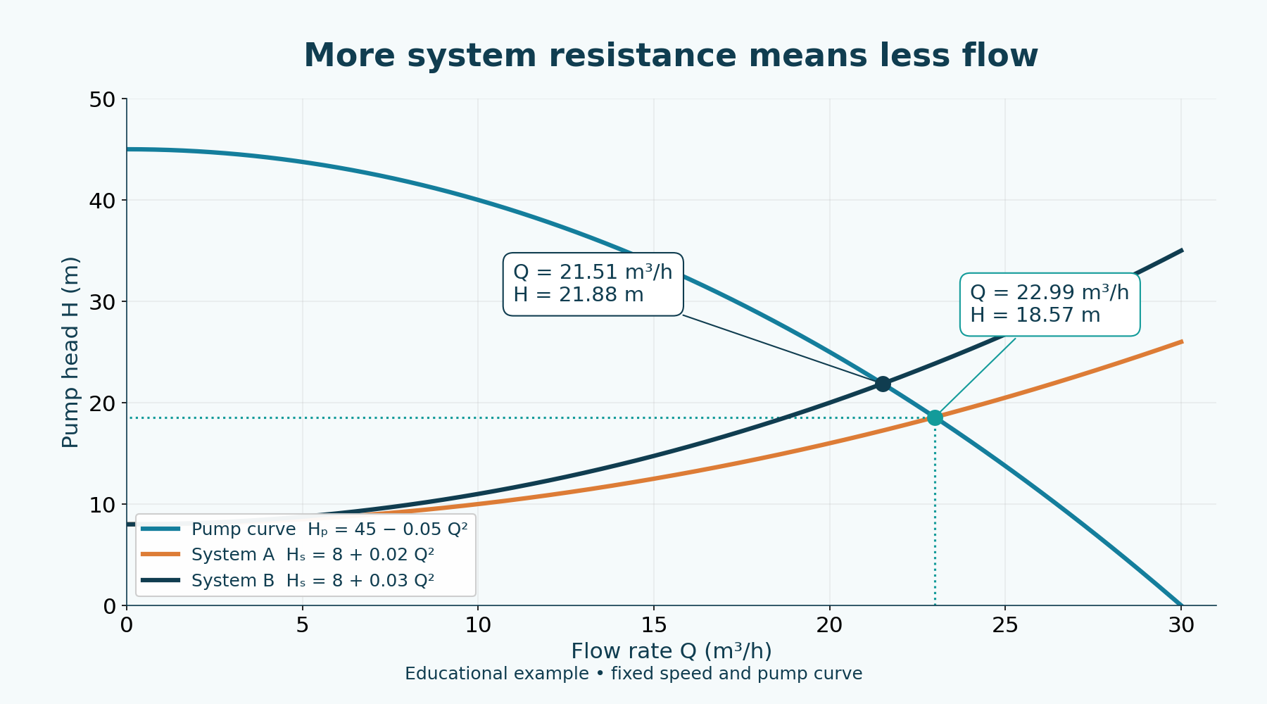
Keeping the pump unchanged, we alter only the system to H_s = 8 + 0.03 Q². Equality gives Q = √(37/0.08) = 21.505813 m³/h and H = 21.875 m. Flow decreases by about 6.5%, while head at the operating point rises. Expecting the previous flow from an installation with a different demand makes no sense.
Even with lower flow, hydraulic power in this model increases to approximately 1.282 kW, and shaft power to 1.972 kW if we artificially keep η_p = 65%. There is no general rule that every reduction in flow decreases power. Real power and efficiency curves can have different shapes, and efficiency itself varies with the operating point.
A discharge valve can change the resistance curve; a suction restriction also changes losses and reduces available NPSH. These effects are not equivalent. The mini-exercise compares curves without prescribing valve operations or turning throttling into an automatic selection solution.
| Result | k = 0.02 | k = 0.03 |
|---|---|---|
| Q | 22.990681 m³/h | 21.505813 m³/h |
| H | 18.571429 m | 21.875000 m |
| η_p in the model | Constant 65% | Constant 65% |
BEP is a point; the operating range must be defined
BEP means Best Efficiency Point: the point of maximum efficiency for the speed and impeller considered. The efficiency curve identifies it. Near design conditions, relative hydraulic behavior is often better; this does not guarantee freedom from vibration, loads or wear.
The preferred operating region, POR, and allowable operating region, AOR, are distinct from BEP. Limits depend on construction and operating constraints, including loads, heating, cavitation and vibration. The manufacturer and application criteria must define the range; we do not adopt a universal percentage of flow for every pump.
The 23 m³/h point in this exercise has not been identified as BEP. We have a head curve and an assumed constant efficiency, not a real efficiency curve. In the lab, changing η_p changes shaft power but does not move the H–Q intersection: the two curves remain unchanged.
NPSH: how much suction head remains above vapor pressure?
NPSH is the absolute total head at the suction reference above the head corresponding to the fluid’s vapor pressure, expressed in meters of liquid. Available NPSH, NPSH_a, belongs to the installation; required NPSH, NPSH_r, is supplied for the pump under specified conditions. They are not simply two gauge pressures read and subtracted.
For an open reservoir with a large surface and negligible surface velocity, a form derived from Bernoulli is NPSH_a = p_atm,abs/(ρg) + z − h_f,s − p_v,abs(T)/(ρg). Elevation z is the surface elevation minus the suction datum, normally the impeller center in this horizontal example: positive when the surface is above it. h_f,s includes losses along the suction path only.
The pressures in this expression are absolute. Local atmospheric pressure, temperature and vapor pressure, reservoir level and losses influence the result. Higher temperature can raise vapor pressure; increasing suction losses reduce available head. We do not subtract velocity head again after using the balance from the surface, because NPSH involves total head.
NPSH3 is a test criterion associated with a 3% drop in head, or first-stage head in a multistage pump, at specified flow and speed. It already allows a cavitation effect and is not a no-bubble limit. The Hydraulic Institute’s public explanation of the 2024 edition of ANSI/HI 9.6.1 clarifies the reference to manufacturer-supplied NPSH_r, equal to or greater than tested NPSH3. We do not treat these terms as universally identical.
A positive NPSH margin still does not approve an installation
In the separate mini-example, NPSH_a = 3.2 m and NPSH_r = 2.6 m give a difference of 0.6 m and a ratio of approximately 1.23. These numbers only illustrate the comparison. The required margin depends on the pump, fluid, operating range and application criteria; 0.6 m is not universal approval.
The lab uses another explicit assumption: NPSH_r(Q) = 1.6 + 0.0025 Q², a curve created for teaching with no catalog origin. At 22.990681 m³/h it gives 2.921429 m; with NPSH_a held at 3.2 m, the difference is 0.278571 m. This curve does not correspond to the mini-example’s fixed required value of 2.6 m.
In a real installation, available NPSH can also vary with flow and transients. Holding NPSH_a constant while varying a synthetic required curve illustrates relationships rather than quantitatively predicting cavitation. The simulator distinguishes negative, zero and positive comparisons and states that sufficiency has not been assessed; it does not issue a safe-operation seal.
Hydraulic Institute — Understanding the 2024 Updates to ANSI/HI 9.6.1 →

Cavitation: vapor bubbles, collapse and damage
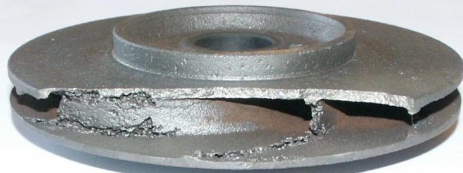
Local pressure can fall enough to allow vaporization near the impeller inlet. Vapor cavities move to higher-pressure regions and collapse. Repetition can compromise performance and cause erosion, especially near surfaces exposed to collapse.
Gravel-like noise, vibration and loss of performance are possible signs; damage to the impeller, seals and bearings can shorten service life. The documented photograph of an impeller with damage attributed to cavitation helps visualize a real consequence but does not represent the exercise’s pump.
These symptoms do not diagnose cavitation on their own. Air ingress, recirculation, misalignment and support problems can also cause noise or vibration. NPSH, suction conditions, operating range and evidence must be examined together. Lack of water does not explain all cavitation, and an apparently full circuit does not prove sufficient availability.
cavitation-photo.webp — Wikimedia Commons / source and author →

Installation errors: the suction path deserves attention
Long suction lines, unsuitable diameter, many fittings and high-loss filters can consume part of the available head. Low level or a large elevation difference between surface and pump also changes the balance. Air ingress and priming conditions depend on the installation and equipment type.
Speed different from that specified, an incompatible impeller, selection outside the anticipated range and different fluid conditions can modify performance. Diagnosis compares observed conditions with assembly documentation. The cause cannot be concluded from motor temperature, sound or a photograph alone.
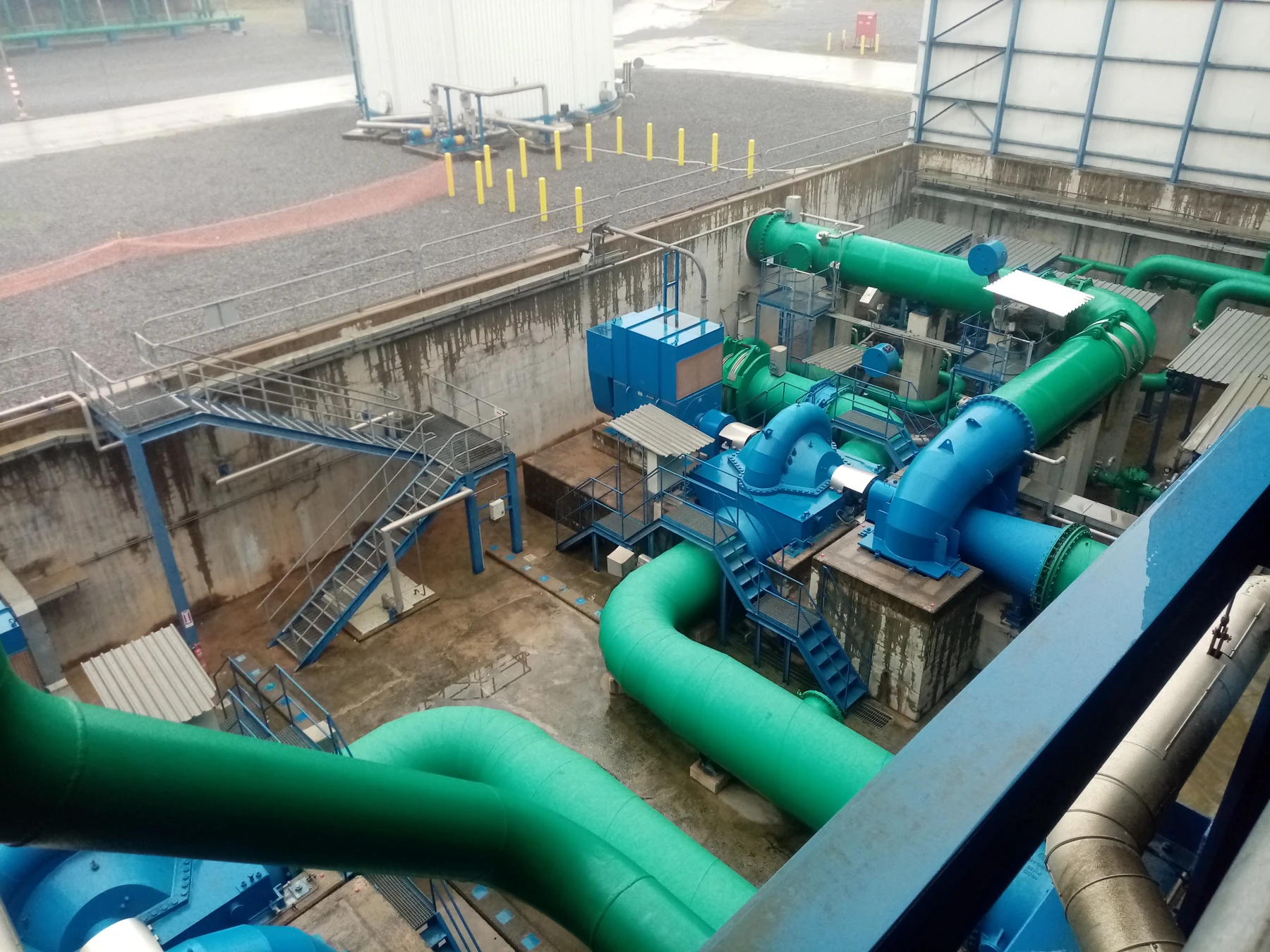
The image of a cooling pump installation shows that the assembly operates alongside pipes, connections, supports and maintenance access. Design must consider the system and its life cycle, as the DOE guide emphasizes. We do not infer losses, NPSH or compliance from the photographed installation.
installation-photo.webp — Wikimedia Commons / source and author →

Licença / License / Licencia: CC BY-SA 4.0 →
DOE — Improving Pumping System Performance, Second Edition — DOE/GO-102006-2079 →
From piping to the exchanger and AI cooling
Pipe pressure loss forms part of the system curve; a heat exchanger also adds a hydraulic demand. Increasing thermal area alone does not determine its pressure drop: channels and distribution matter. The piping, exchanger and pump articles thus describe connected parts of the same circuit.
In data-center liquid cooling, reliable circulation helps transport heat from cold plates and CDUs. Flow and heat capacity must match the energy path, but the point calculated here is not a specification for that system. Materials, redundancy, control and component limits remain decisions for the real design.
Interactive lab: find and interpret the operating point
Change shutoff head, pump coefficient, static head and system coefficient. Compare the intersection and powers. Then change pump efficiency: shaft power changes without shifting this model’s head curves. The equivalent table lets you read values without relying on colors.
Try increasing k from 0.02 to 0.03 and check the flow reduction. Raise static head to shutoff head: the model stops predicting positive flow. Observe the comparison between available NPSH and the synthetic curve, remembering that the result does not assess the necessary margin.
Controls and notices are translated; calculations run locally in the browser. Standalone HTML, Python and CSV allow the exercise to be reproduced. Without JavaScript, examples and static charts remain available, but fields do not update results.
Lab: pump curve and system curve
Water model (ρ = 1000 kg/m³; g = 9.81 m/s²), with fixed speed and hypothetical curves. Local calculations; inputs are not transmitted.
Educational simulation. Efficiency refers to the pump; electric power is not calculated. Available NPSH is a constant input, and required NPSH is a synthetic curve without catalogue provenance.
- Operating flow (m³/h)
- 22.991
- Operating head (m)
- 18.571
- Hydraulic power (kW)
- 1.163
- Shaft power (kW)
- 1.790
- Educational NPSH_r at the point (m)
- 2.921
- NPSH_a − NPSH_r difference (m)
- 0.279
Positive educational comparison: NPSH_a > NPSH_r at the point. Margin adequacy is not assessed. This result does not certify absence of cavitation; consult pump and application data and criteria.
Equivalent curve table
| Q (m³/h) | Pump H (m) | System H (m) |
|---|---|---|
| 0.000 | 45.000 | 8.000 |
| 15.000 | 33.750 | 12.500 |
| 22.991 | 18.571 | 18.571 |
| 30.000 | 0.000 | 26.000 |
H_p = H₀ − aQ²; H_s = H_est + kQ²; NPSH_r = b₀ + cQ². Q is in m³/h in these curves. P_h = ρg(Q/3600)H; P_shaft = P_h/η_p.
η_p is held constant; no efficiency curve is provided to identify BEP. The model does not determine actual losses, speed, vapour pressure or adequate NPSH margin. Ranges are lab limits, not equipment limits.
Open the standalone PT/EN/ES simulator →
The pump meets the installation and the fluid’s limits
Reading the H–Q curve is only the beginning. Flow depends on its intersection with the system; power depends on transported energy and efficiencies; suction behavior requires comparing NPSH under relevant conditions. A coherent calculation must keep these boundaries separate.
A centrifugal pump does not work alone: it meets the installation, fluid and its physical limits. That interaction determines actual flow, efficiency — and, when something goes wrong, cavitation.
Frequently asked questions
How do you find a pump’s operating point?
Compare the pump head curve with the system demand curve using the same units and conditions. Their intersection determines predicted flow and head. In the example, equating 45 − 0.05 Q² to 8 + 0.02 Q² gives 22.99 m³/h and 18.57 m. Real curves depend on speed, impeller, fluid and installation; flow cannot be selected by looking only at motor power.
What are available and required NPSH?
Available NPSH describes the absolute total head at the suction reference above the liquid’s vapor pressure. It depends on the installation. Required NPSH is stated for the pump under specified conditions. Comparison must consider an appropriate margin and the manufacturer’s reference; NPSH3, linked to a 3% test head drop, does not mean cavitation is absent. A positive difference alone does not approve selection.
What causes cavitation in a centrifugal pump?
Local vaporization can occur when pressure falls to the level associated with the fluid’s vapor pressure. Cavities can collapse in higher-pressure regions, causing noise, performance degradation and erosion. Temperature, level, atmospheric pressure and suction losses influence available NPSH. Cavitation should not be confused with all air ingress or every noise: similar symptoms require combined diagnosis.
Why can a pump be running yet fail to pump properly?
A turning motor does not establish adequate flow. High resistance, incompatible selection, different speed, suction conditions, air in the flow path and other problems can change the result. In the lab model, static head equal to or greater than shutoff head eliminates predicted positive flow. In a real installation, conditions and assembly data must be compared without attributing the cause to a single sign.
What is the difference between hydraulic, shaft and electrical power?
Hydraulic power is delivered to the liquid: ρ g Q H, with Q in m³/s. Shaft power includes pump losses and is obtained by dividing hydraulic power by pump efficiency. Electrical power also includes motor and drive losses. In the example, 1.16349 kW hydraulic power and 65% pump efficiency give 1.78999 kW at the shaft; electrical power was not determined.
Is the operating point always the BEP?
No. BEP is the point of maximum efficiency for a specified speed and impeller. The pump–system intersection may be far from it. POR and AOR describe operating regions, with limits defined for the equipment and application. The exercise does not provide an efficiency curve; therefore, its calculated 23 m³/h cannot be identified as BEP.
Does available NPSH greater than required guarantee no cavitation?
Not on its own. Comparison must use the manufacturer’s stated reference and a margin appropriate to the service. Criteria, variable conditions, fluid and operating range must be considered. NPSH3 already corresponds to test head degradation, and required NPSH should not be treated as universally identical to it. The simulator displays numerical differences without certifying freedom from bubbles, damage or risk.
Does increasing circuit resistance always reduce consumption?
No. Increasing resistance shifts the intersection and may reduce flow, but head and efficiency also change. In the model presented, changing k from 0.02 to 0.03 reduces flow and raises calculated hydraulic power. Real equipment requires reading the power curve and assembly characteristics. A conclusion about electrical energy also needs to consider motor, drive, control and operating time.
References
- Hydraulic Institute — Pump CurvesHydraulic Institute
- Hydraulic Institute — System CurvesHydraulic Institute
- Hydraulic Institute — Combined Pump and System CurvesHydraulic Institute
- Hydraulic Institute — Definitions: NPSHA, NPSHR and NPSH3Hydraulic Institute
- Hydraulic Institute — Pump PrinciplesHydraulic Institute
- Hydraulic Institute — Understanding the 2024 Updates to ANSI/HI 9.6.1Hydraulic Institute
- KSB Lexicon — NPSHKSB
- DOE — Improving Pumping System Performance, Second Edition — DOE/GO-102006-2079U.S. Department of Energy
- pump-photo.webp — photographic provenanceWikimedia Commons / Real centrifugal pump and electric motor assembly. Photo: HopuWiki / Wikimedia Commons, CC BY-SA 4.0. Resized and converted to WebP.
- installation-photo.webp — photographic provenanceWikimedia Commons / Cooling-water pumps and pipework at Gebze power plant. Photo: Harald the Bard / Wikimedia Commons, CC BY-SA 4.0. Resized and converted to WebP.
- cavitation-photo.webp — photographic provenanceWikimedia Commons / Pump impeller with cavitation damage, as identified by its author. Photo: Klausbärbel / Wikimedia Commons, CC BY-SA 3.0. Converted to WebP; original resolution retained.