
Learn to size heat exchangers using LMTD and effectiveness–NTU. Explore worked examples, charts and an interactive simulator.
Can cold water leave hotter than the hot outlet?
Yes. In a counterflow heat exchanger, cold water can leave at a higher temperature than the hot-water outlet. The apparent paradox disappears when we identify where each outlet is: they are at opposite ends. The direction of heat transfer depends on the fluid temperatures at the same physical location, not a comparison between two distant sensors.
We will explore this distinction and answer two engineering questions. If we know area, flow rates and inlet temperatures, how much heat does the equipment transfer? If we specify an outlet temperature, how much area do we need? The effectiveness–NTU method answers the first; the logarithmic mean temperature difference, LMTD, helps solve the second.
This edition examines the exchanger used in the CDUs discussed in our article on liquid cooling for AI data centers. The lab, however, uses industrial water entering at 80 °C and 20 °C. These hypothetical inputs were chosen for teaching: they do not represent server temperatures, a real development or equipment selected from a catalog.
What exactly is a heat exchanger?
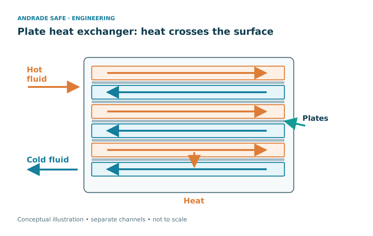
In the equipment studied here, two fluids exchange energy through a surface that separates them. The hot fluid heats the wall; energy crosses the material by conduction and reaches the cold fluid. Liquid movement promotes convection on each side. There is no intentional mixing between the streams, although integrity failures can compromise that separation.
This principle appears in industrial heat recovery, process heating, HVAC, chilled-water systems and refrigeration. In a liquid-to-liquid CDU, the exchanger thermally connects the electronic-component circuit to the facility circuit. Other equipment, such as cooling towers, may involve direct contact and evaporation; its description and models differ from this article’s single-phase example.
The exchanger does not create energy or independently carry heat to its final destination. Pumps maintain circulation; controls adjust operation; another device or thermal use receives the energy. Calculating thermal area is therefore one part of the design and must work alongside hydraulics, materials, integrity and maintenance.
Plates, shell and tubes: geometry matters
Plate heat exchangers arrange thin surfaces into alternating channels for the fluids. Corrugations and flow distribution influence convection, pressure loss and cleaning. The area can be compact, and certain configurations allow a small temperature approach. Alfa Laval’s official animation helps visualize adjacent channels in counterflow; it illustrates operation rather than confirming U for our exercise.
A gasketed plate assembly may allow opening and inspection, depending on the model. Brazed or welded equipment offers other maintenance options and limitations. Compatibility among fluid, plates and gaskets, together with design pressure and temperature, guides selection. A plate heat exchanger is not a universal guarantee of suitability or easy cleaning.
In a shell-and-tube unit, one stream passes through tubes and the other flows through the shell. Passes, baffles, arrangement and the ability to remove the bundle affect performance and access. In a double-pipe exchanger, one stream travels through the inner pipe and the other through the annular space, making ideal flows easier to understand. Real comparisons must consider area, fouling, space, life-cycle cost and permissible pressure drop.
Alfa Laval — How gasketed plate heat exchangers work (official animation) →
Energy balance: heat released and heat received
We assume steady state, liquid water, constant specific heat capacity, no work within the exchanger and negligible external heat losses. Under these conditions, the power released by the hot stream equals that received by the cold stream: Q̇ = ṁ_h c_p,h (T_h,in − T_h,out) = ṁ_c c_p,c (T_c,out − T_c,in). The unit of Q̇ is W; it represents energy per unit time, not an accumulated quantity of heat.
The heat capacity rate is C = ṁ c_p, in W/K. A stream with a larger C changes temperature less when receiving or releasing the same power. Specific heat capacity c_p is a fluid property; C also includes flow rate. We identify C_min and C_max to compare streams independently of which one is hot.
For water with c_p = 4180 J/(kg·K), flow rates of 1.2 kg/s and 1.0 kg/s give C_h = 5016 W/K and C_c = 4180 W/K. The cold stream has the minimum capacity, and C_r = C_min/C_max = 0.83333. A temperature difference of 1 K has the same magnitude as 1 °C; we use differences in K in the balances and terminal temperatures in °C.
| Quantity | Unit | Interpretation |
|---|---|---|
| Q̇ | W or kW | Transferred thermal power |
| ṁ | kg/s | Mass flow rate |
| c_p | J/(kg·K) | Specific heat capacity |
| C = ṁ c_p | W/K | Stream heat capacity rate |
| U | W/(m²·K) | Overall coefficient on the adopted area basis |
| A | m² | Effective area consistent with U |
| ε and NTU | Dimensionless | Effectiveness and relative thermal size |
| LMTD | K | Logarithmic mean of terminal differences |
Counterflow and parallel flow
In parallel flow, both fluids enter at the same end and travel in the same direction. The temperature difference is large at the inlet and decreases as the temperatures converge. The outlets are side by side: in a simple single-phase exchanger without external sources, the cold stream cannot exceed the hot stream at that end.
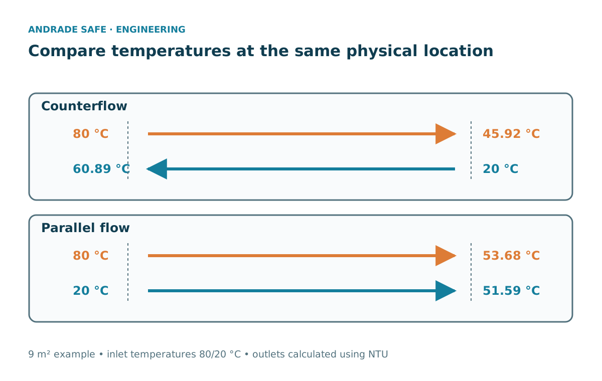
In counterflow, the fluids enter at opposite ends. Where the cold stream leaves, the hot stream is entering; where the hot stream leaves, the cold stream is entering. This can maintain a useful driving force along the surface and enable greater heat recovery with the same area and all other assumptions unchanged.
Saying counterflow is more efficient is insufficient. The thermal comparison requires the same capacities, U and area and does not automatically assess pumping consumption or cost. Passes and channels in real equipment may also differ from ideal counterflow. The thermal benefit does not remove the need for mechanical integrity and hydraulic compatibility.
LMTD: why does the mean have to be logarithmic?
The temperature difference between streams changes along the exchanger. A square meter near a large temperature difference does not transfer the same power as one near a small approach for the same U. Under the model’s assumptions, integrating the balance gives ΔT_lm = (ΔT_1 − ΔT_2)/ln(ΔT_1/ΔT_2). Substituting an arithmetic mean produces a different result.
In counterflow, we compare terminals that actually occupy the same end: ΔT_1 = T_h,in − T_c,out and ΔT_2 = T_h,out − T_c,in. In parallel flow: ΔT_1 = T_h,in − T_c,in and ΔT_2 = T_h,out − T_c,out. The end numbering can be reversed without changing the mean, provided each local comparison is correct.
The area relationship is Q̇ = U A F ΔT_lm. For the pure ideal arrangements in this lab, F = 1. Multipass, crossflow and shell-and-tube configurations require an appropriate factor or topology-specific relationships. F = 1 is not a universal assumption for every exchanger.
Both terminal differences must be positive in the calculation presented. When they are equal or very close, the direct expression tends toward 0/0; its limit is the temperature difference itself. A calculator must handle this continuous case rather than reject a physically possible condition or display an undefined result.
MIT OpenCourseWare — Introduction to Engineering Heat Transfer, section 8 →
Effectiveness–NTU: when the outlets are still unknown
If we know inlet temperatures, flow rates, U and area, the outlets need to be predicted. First we calculate Q̇_max = C_min (T_h,in − T_c,in). This is the model’s reference thermal limit, not the guaranteed duty of a device. Effectiveness ε = Q̇/Q̇_max indicates what fraction of that potential is used.
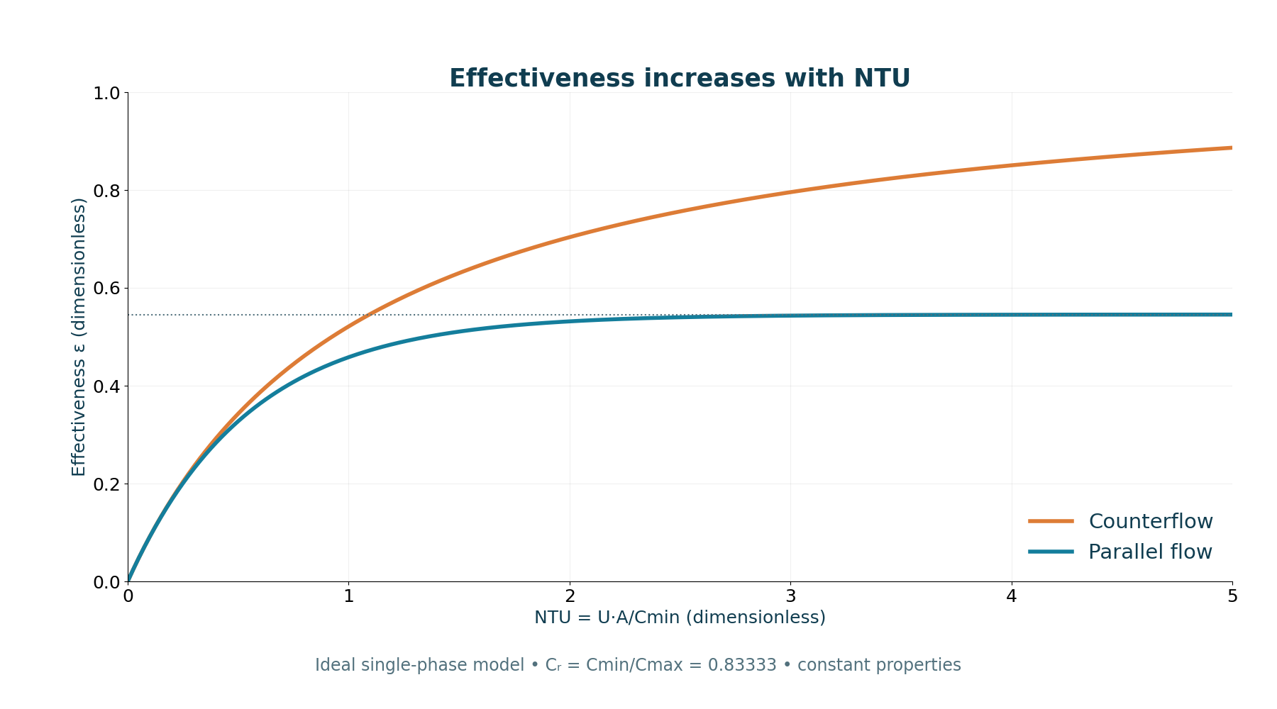
The number of transfer units is NTU = U A/C_min, a dimensionless quantity. It relates the surface’s transfer capability to the capacity of the limiting stream. Increasing area or U increases NTU when C_min remains constant; transferred heat grows with progressively diminishing returns. Behavior also depends on C_r and the arrangement.
For ideal parallel flow: ε = [1 − exp(−NTU(1 + C_r))]/(1 + C_r). For counterflow with C_r ≠ 1: ε = [1 − exp(−NTU(1 − C_r))]/[1 − C_r exp(−NTU(1 − C_r))]. When C_r = 1, we use the limit ε = NTU/(1 + NTU). Then Q̇ = ε Q̇_max, T_h,out = T_h,in − Q̇/C_h and T_c,out = T_c,in + Q̇/C_c.
These relationships describe the two chosen ideal single-phase arrangements. They should not be applied indiscriminately to evaporators, condensers, multiple passes or other geometries. For the same valid model, LMTD and NTU must agree; this agreement is a mathematical check, not validation of a detailed engineering design.
NPTEL — Heat Exchangers, Lecture 36: effectiveness and NTU →
Exercise 1: what happens in a 9 m² exchanger?
Consider hot water entering at 80 °C, cold water at 20 °C, flow rates of 1.2 and 1.0 kg/s respectively, and c_p = 4180 J/(kg·K) for both. We assume U = 850 W/(m²·K) and effective area A = 9.0 m². U is a constant editorial assumption; it was neither measured nor taken from a product catalog.
With C_min = 4180 W/K and C_r = 0.83333, NTU = 850 × 9/4180 = 1.83014. The reference maximum is Q̇_max = 4180 × (80 − 20) = 250800 W = 250.8 kW. Applying each arrangement’s relationships gives the results below.
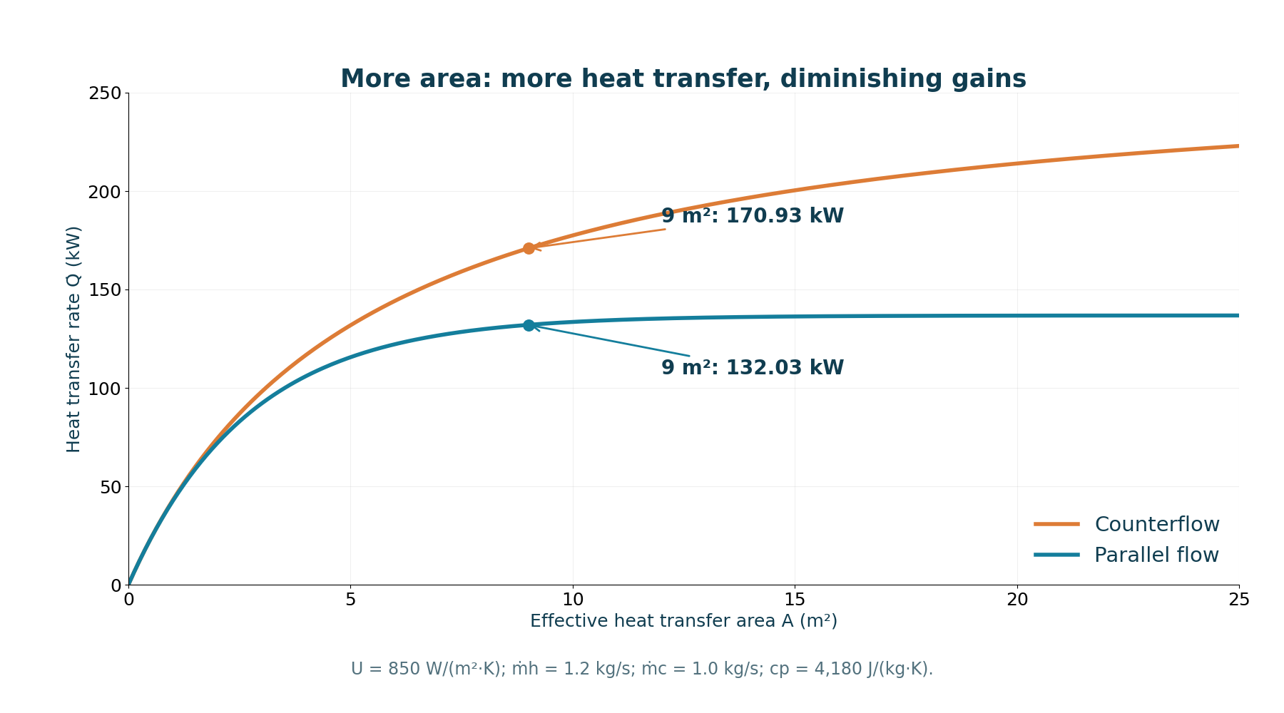
Counterflow transfers 170.93 kW, compared with 132.03 kW for parallel flow: about 29.5% more in this scenario with the same area and U. This compares transferred thermal power, not a percentage reduction in electricity consumption. The hot- and cold-side heat duties must balance before interpreting efficiency.
| Result | Counterflow | Parallel flow |
|---|---|---|
| C_h / C_c | 5016 / 4180 W/K | 5016 / 4180 W/K |
| C_r | 0.83333 | 0.83333 |
| NTU | 1.83014 | 1.83014 |
| Q̇_max | 250.80 kW | 250.80 kW |
| ε | 0.68152 | 0.52642 |
| Q̇ | 170.93 kW | 132.03 kW |
| T_h,out | 45.92 °C | 53.68 °C |
| T_c,out | 60.89 °C | 51.59 °C |
| LMTD | 22.34 K | 17.26 K |
| U A LMTD | 170.93 kW | 132.03 kW |
A cold outlet at 60.89 °C does not violate thermodynamics
At the end where the cold stream leaves at 60.89 °C, the hot stream enters at 80 °C: the local temperature difference is 19.11 K. At the other end, the hot stream leaves at 45.92 °C and the cold stream enters at 20 °C: the difference is 25.92 K. The fluids maintain the hot–cold ordering at every location, although outlet temperatures measured in different places appear reversed.
The counterflow energy check is 5016 × (80 − 45.923847) ≈ 170926 W and 4180 × (60.891384 − 20) ≈ 170926 W. With unrounded terminal differences, LMTD = 22.343266 K and 850 × 9 × 22.343266 ≈ 170926 W. In parallel flow, LMTD = 17.258256 K reproduces 132026 W. Small discrepancies when repeating calculations with only two decimal places arise from rounding.
A positive driving force must exist along the route, not just in the highlighted numbers. The temperature chart and arrows help avoid interpreting the cold stream as having overtaken the hot stream at the same location. This spatial understanding is just as important as correctly substituting values into formulas.
Exercise 2: what area heats the water to 55 °C?
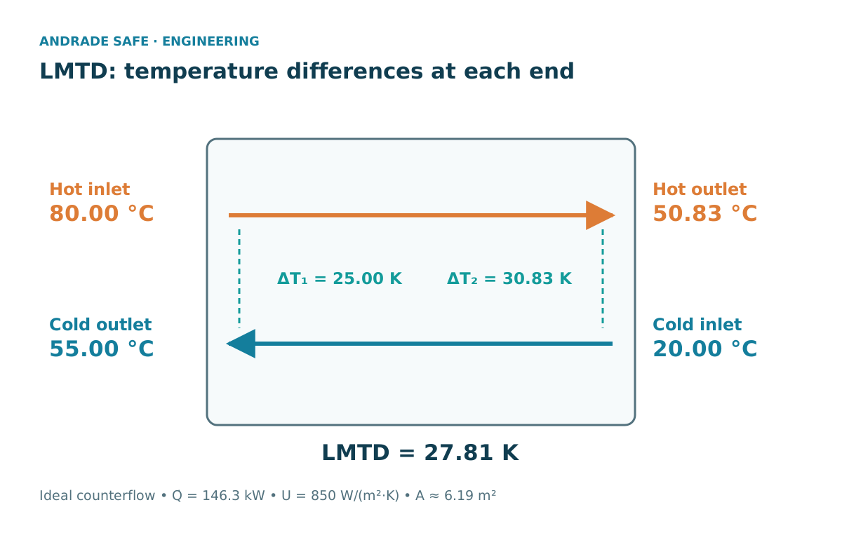
Now retain the inlet temperatures, flow rates, c_p and U but specify T_c,out = 55 °C in counterflow. The required power is Q̇ = 1.0 × 4180 × (55 − 20) = 146300 W. On the hot side, T_h,out = 80 − 146300/5016 = 50.83333 °C. The balance determines this outlet; we cannot choose both outlets independently.
The correct differences are ΔT_1 = 80 − 55 = 25 K and ΔT_2 = 50.83333 − 20 = 30.83333 K. The logarithmic mean is 27.814794 K. With F = 1, A = 146300/(850 × 27.814794) = 6.187989 m², or 6.19 m². This is the model’s ideal thermal area, without margin, geometry or catalog selection.
Reinserting the unrounded area into the NTU method gives NTU = 1.258323, ε = 0.583333 and a cold outlet at 55.00 °C. Both methods therefore describe the same condition. Entering 6.19 m² gives a slightly different outlet because the area was rounded. Retain precision internally and round only the presentation.
The target is unattainable in simple parallel flow with these inlets and capacities: the calculated hot outlet would be 50.83 °C, below the cold stream’s 55 °C at the same end. The asymptotic limit of both outlets is approximately 52.73 °C. No finite area in this parallel-flow model reaches 55 °C; increasing A does not solve the problem.
| Step | Result |
|---|---|
| Required Q̇ | 146.30 kW |
| T_h,out from balance | 50.83333 °C |
| ΔT_1 / ΔT_2 | 25.00000 / 30.83333 K |
| LMTD | 27.81479 K |
| Unrounded area | 6.187989 m² |
| Displayed area | 6.19 m² |
| ε from NTU check | 0.583333 |
| T_c,out from check | 55.00 °C |
Overall coefficient U: resistances and area basis
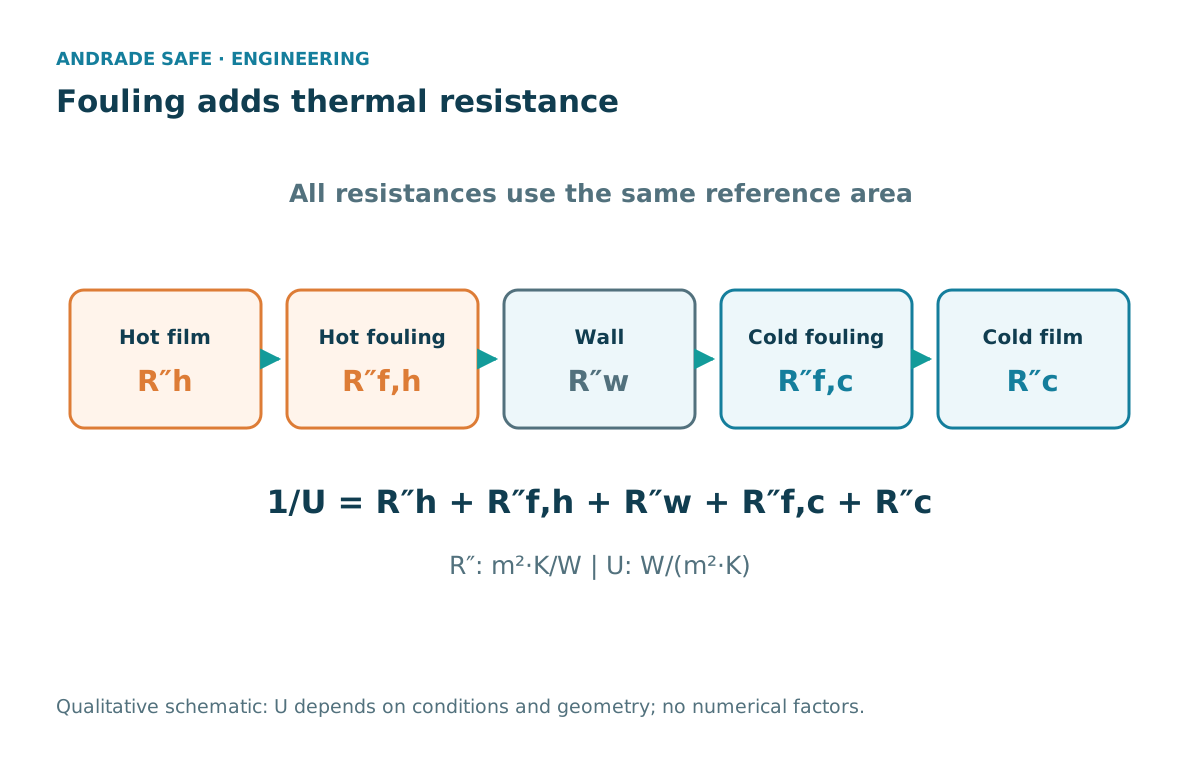
Heat encounters resistances in series: the hot-side convective film, the wall, possible deposits and the cold-side convective film. In a simplified planar representation using the same area basis, 1/U can be written as 1/h_h + R_f,h + δ/k + R_f,c + 1/h_c. Fouling resistances are expressed in m²·K/W in this formulation. Without a consistent basis, adding these terms does not define the U used in the equation.
In tubes, internal and external areas differ, and conduction through the cylindrical wall includes geometry. U must be identified as based on internal or external area, and resistances converted consistently. In plates, corrugations, channels and flow distribution enter correlations and manufacturer selection.
U also depends on velocities, viscosity, properties, temperatures and cleanliness. Holding it at 850 W/(m²·K) makes the teaching comparison transparent but does not predict its real evolution. Reducing U in the simulator is a sensitivity analysis; it does not turn the result into a fouling estimate for specific equipment.
NPTEL — Lecture 34: overall coefficient and area reference →
Does more area make the pump work harder?
There is no universal relationship between thermal area and pump power. Adding plates may create more parallel channels or change length, cross section, velocity or distribution. Depending on the configuration, pressure drop may decrease or increase. The Q̇ versus A chart keeps U and flow rates constant; it is not a hydraulic curve.
To estimate pumping, we need volumetric flow, total pressure difference and efficiency: P_el ≈ Δp V̇/η_overall. U and A do not provide these inputs. Final selection considers pressure-loss limits on both sides, materials, gaskets, design pressure and temperature, accessibility and, where relevant to the pumping system, cavitation conditions.
Thermally sufficient equipment may be unsuitable because of corrosion, incompatibility, pressure or maintenance. The calculated area also does not establish wall thickness, connection strength, supports or integrity. Thermal and mechanical engineering must arrive at the same operational solution.
DOE — Industrial Steam System Heat-Transfer Solutions — DOE/GO-102003-1738 →
Fouling, water quality and maintenance
Deposits may add thermal resistance and narrow flow passages. The result may be less heat exchange, greater pressure drop or altered distribution among channels. DOE links fouling to equipment efficiency and life-cycle cost and discusses side-stream filtration as an option in certain cooling-tower systems.
This does not mean a cooling-tower technology should automatically be applied to a CDU. Fluid quality, materials, open or closed circuits, treatment and supplier recommendations change the problem. Fouling factors adopted for selection need a source and justification; we do not add a fictional R_f to the exercise.
Cleaning in place, or CIP, is a maintenance option in suitable configurations with defined procedures and conditions. It is introduced here as a concept. Trends in temperatures, differential pressure and flow rates help track performance, but an inferred drop in U alone does not diagnose the cause. Instrumentation, balances and operating conditions need to be examined together.
How does this connect to CDUs in AI data centers?
In a liquid-to-liquid CDU, the exchanger transfers energy between separate circuits. The sides may have different fluids, flow rates and quality requirements, as well as temperature and pressure limits. The achievable thermal approach depends on U, area, capacities and operating conditions; it should not be confused with the temperature rise of a single stream.
The previous article follows cold plates, manifolds, pumping and heat rejection. This lab explores one part of that route in greater depth. Water at 80 °C and 20 °C does not specify the Mumbai project or another commercial data center. Operational continuity, control, leaks, filtration, sensors and contingencies remain questions for the complete system.
Interactive experiment: watch the methods agree
Change area, U, both flow rates and inlet temperatures, then select parallel flow or counterflow. The lab displays power, effectiveness, NTU, outlets and LMTD; the curve compares the two arrangements with the other inputs held constant. The equivalent table lets you read values without depending on colors or the chart.
Try three experiments: restore 9 m² and compare the arrangements; use the calculated area of 6.187989 m² and look for 55 °C at the cold outlet; equalize the flow rates to obtain C_r = 1 and observe continuity in the counterflow relationship. Numeric fields allow values between slider steps. Inputs outside the lab’s domain do not produce results.
Calculations run in the browser without sending your inputs to a facility. The standalone HTML has a PT/EN/ES selector, and the Python code reproduces the equations without external libraries. The package includes figures and a scenario CSV. Without JavaScript, the exercises and figures remain available; the controls do not update the prediction.
Which heat exchanger transfers more heat?
Change the assumptions; calculations run in the browser without sending values to external systems.
Educational steady-state single-phase water model, constant heat capacity (4,180 J/kg·K), constant U, no external losses, pressure drop, fouling, phase change or actual exchanger geometry. Not for final equipment design.
- Heat transfer rate (kW)
- 170.926
- Effectiveness (ε)
- 0.68152
- NTU
- 1.83014
- Hot outlet (°C)
- 45.924
- Cold outlet (°C)
- 60.891
- Log mean temperature difference (K)
- 22.34327
- U A LMTD check (kW)
- 170.926
C_h = 5,016.0 W/K; C_c = 4,180.0 W/K; C_r = 0.83333; Q̇_max = 250.800 kW.
Equivalent curve table
| A (m²) | Counterflow (kW) | Parallel flow (kW) |
|---|---|---|
| 0.000 | 0.000 | 0.000 |
| 3.000 | 98.072 | 92.094 |
| 6.188 | 146.300 | 123.179 |
| 9.000 | 170.926 | 132.026 |
| 15.000 | 200.393 | 136.290 |
| 20.000 | 214.013 | 136.721 |
Rounded parallel-flow outlets may appear equal near the limit. LMTD retains the analytical terminal difference to avoid numerical cancellation.
C = ṁ c_p; NTU = U A/C_min; Q̇ = ε C_min (T_h,in − T_c,in); Q̇ = U A LMTD; c_p = 4180 J/(kg·K).
F = 1 only for the ideal arrangements in this model. Ranges are educational limits, not product limits. The model does not determine pumping power, design pressure or equipment selection.
Open the standalone PT/EN/ES simulator →
Download the reproducible Python model →
Two methods, one thermodynamics
LMTD helps determine area for a desired, physically possible outlet condition. Effectiveness–NTU helps predict performance when inlets, capacities and surface are known. The energy balance connects the methods and prevents inconsistent choices of outlet temperatures.
In the examples, counterflow explains why the cold outlet exceeds the hot outlet, and NTU results agree with U A LMTD. This verification strengthens understanding but does not replace a catalog, hydraulic analysis or the final thermal and mechanical design. In a heat exchanger, geometry brings the fluids close together; the equations reveal how much energy can actually cross that boundary.
Frequently asked questions
What is a heat exchanger, and how does it work?
It is equipment that transfers energy between streams at different temperatures. In this article’s models, fluids are separated by a wall: convection on each side and conduction through the material form the thermal path. Heat received by one stream equals that released by the other under steady-state assumptions with negligible external losses. Direct-contact or phase-change equipment requires appropriate description and analysis.
How do you calculate heat-exchanger area?
First determine the required power through an energy balance and check that the desired temperatures are physically compatible. Then calculate the arrangement’s terminal differences and LMTD. With U on the same area basis, use A = Q̇/(U F LMTD). F = 1 applies to the two pure ideal arrangements presented. The resulting area is thermal; it does not define geometry, design pressure or final equipment selection.
What is the difference between LMTD and NTU?
LMTD uses known terminal differences and helps size the surface for a desired condition. Effectiveness–NTU uses inlets, heat capacity rates and U A to predict power and outlet temperatures. Both methods must agree when describing the same topology and assumptions. Discrepancies may reveal incorrect temperature pairings, incompatible units, excessive rounding or an effectiveness relationship unsuitable for the equipment.
Can the cold fluid leave hotter than the hot outlet?
Yes, under appropriate counterflow conditions. In the 9 m² example, the cold stream leaves at 60.89 °C and the hot stream at 45.92 °C, at opposite ends. Where the cold stream leaves, the hot stream enters at 80 °C; at the other end, the cold stream enters at 20 °C. The local ordering remains compatible with heat transfer from hot to cold. This outlet reversal is impossible in the example’s simple parallel flow.
What is thermal effectiveness?
Effectiveness is ε = Q̇/Q̇_max, with Q̇_max = C_min(T_h,in − T_c,in) in the model presented. It compares transferred power with the potential limited by inlets and the smaller heat capacity rate. It is dimensionless and depends on NTU, the capacity ratio and arrangement. It is not COP, electrical efficiency or a pump-consumption indicator; greater effectiveness may come with other design demands.
What reduces heat-exchanger performance?
Fouling, flow changes, properties different from predictions, uneven distribution and inlet conditions can change performance. Deposits may affect both thermal and hydraulic resistance. Comparisons must consider the same load and operating conditions rather than attributing every temperature difference to dirt. Assessment combines balances, temperatures, flows and pressures with maintenance and fluid quality appropriate to the equipment.
What is the advantage of a plate heat exchanger?
Plate construction can provide a large area in a compact volume and allow close temperature approaches. Some gasketed models can be opened for inspection and cleaning; brazed and welded models have other characteristics. Selection depends on fluids, materials, pressure, temperature, maintenance and permissible pressure loss. The manufacturer’s animation illustrates operation but does not provide the U assumed in our example or replace technical selection.
Does LMTD apply to evaporators and condensers?
The thermal driving-force concept remains useful, but analysis must reflect phase change, properties and actual conditions. The single-phase balance ṁ c_p ΔT and this lab’s effectiveness relationships should not be applied indiscriminately to condensation and evaporation. Depending on the case, enthalpies, specific relationships and subdivisions by regime are required. Topology and correction-factor validity must also be checked.
References
- MIT OpenCourseWare — Introduction to Engineering Heat Transfer, section 8MIT OpenCourseWare
- NPTEL — Heat Exchangers, Lecture 36: effectiveness and NTUNPTEL
- NPTEL — Lecture 36: counterflow and other configurationsNPTEL
- Alfa Laval — How gasketed plate heat exchangers work (official animation)Alfa Laval
- NPTEL — Lecture 35: LMTD correction factorNPTEL
- NPTEL — Lecture 34: overall coefficient and area referenceNPTEL
- NPTEL — Lecture 34: foulingNPTEL
- DOE — Industrial Steam System Heat-Transfer Solutions — DOE/GO-102003-1738U.S. Department of Energy
- DOE / FEMP — Side Stream Filtration for Cooling TowersDOE / FEMP
- Alfa Laval — The Theory Behind Heat TransferAlfa Laval