
Understand how metal fatigue develops, interpret S–N curves, apply Goodman and Miner, and assess crack growth in components.
Withstanding a load is not the same as withstanding its repetition
A shaft under rotating bending, a bolt or a support subject to vibration may fail after thousands of cycles even though its calculated maximum nominal stress remains below static yield strength. How does this happen? Fatigue is progressive damage under cyclic loading: load history matters as much as the value observed at one instant.
The statement about nominal stress does not mean every microscopic region of the component remained below local yielding. Geometry, notches and defects can concentrate stress; deformation and damage mechanisms in the microstructure are not described solely by a cross-section’s average. Surface condition, environment and residual stresses also enter this history.
Static strength answers a question about capacity under a particular condition. Fatigue assessment follows the effect of repetitions on integrity. We will use contextualized real photographs, entirely synthetic examples and a documented historical case. No calculation in this lab is a test result for a commercial material or approval of a component.

From initial damage to final rupture
In an educational description, failure may involve crack initiation, growth over successive cycles and final rupture of the remaining section. These stages do not necessarily appear as three perfectly visible zones. A component may already contain a defect before entering service; corrosion, manufacturing and loading history change the path.
The propagation region may occupy part of the surface, while another region records final rupture. This helps frame questions but appearance does not replace investigation. Multiple origins, oxidation and rubbing after fracture can change or obscure evidence. A significant crack can also grow without an obvious external sign.
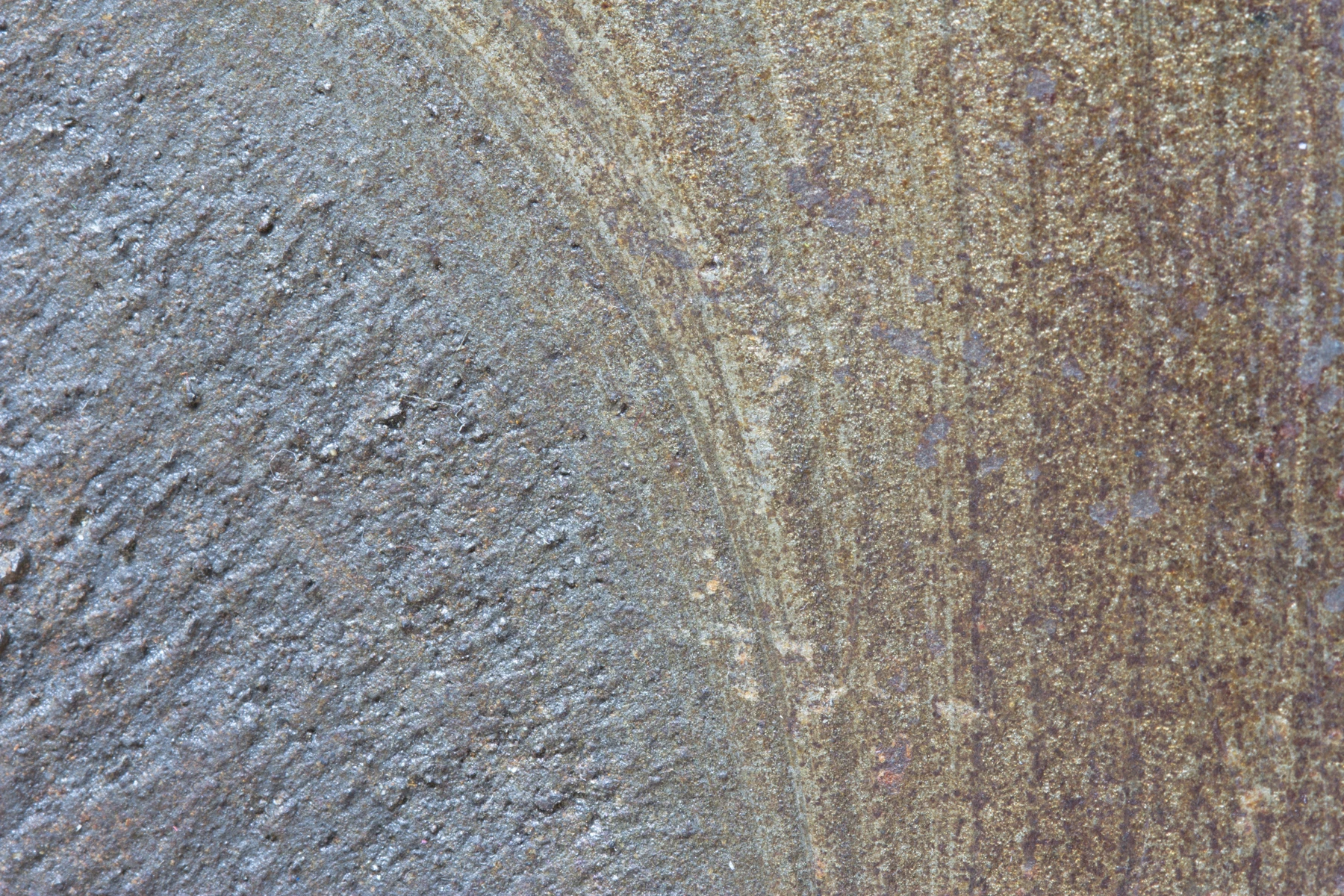
The cover photograph is identified by its author as a fatigue fracture in steel. The zone diagram is a separate conceptual figure; we do not draw striations or an assumed origin over the photograph. Interpretation of each surface must combine loading, material, geometry and appropriate examination.
What is a stress cycle?
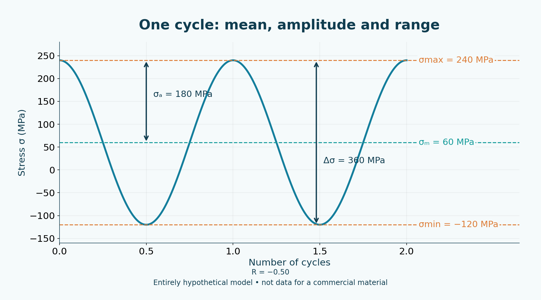
For a cycle with maximum stress σ_max and minimum stress σ_min, we use σ_m = (σ_max + σ_min)/2 for mean stress and σ_a = (σ_max − σ_min)/2 for amplitude. The range is Δσ = σ_max − σ_min = 2σ_a. All have stress units, here MPa. Amplitude and range are not interchangeable in the equations.
With σ_max = 240 MPa and σ_min = −120 MPa, mean stress is 60 MPa, amplitude 180 MPa and range 360 MPa. The ratio R = σ_min/σ_max is −0.50. Under the adopted convention, positive means tension and negative means compression; R is defined this way only when σ_max is nonzero.
A fully reversed cycle has opposite extremes and R = −1; a pulsating cycle with a zero minimum has R = 0. Two histories can have the same amplitude and different means, producing different fatigue responses. Real loading may also be irregular, multiaxial or include stops and transients rather than the sinusoidal form used in the figure.
| Quantity | Expression | Result |
|---|---|---|
| Mean σ_m | (240 − 120)/2 | 60 MPa |
| Amplitude σ_a | (240 + 120)/2 | 180 MPa |
| Range Δσ | 240 − (−120) | 360 MPa |
| Ratio R | −120/240 | −0.50 |
The S–N curve: a test, a life definition and considerable scatter
An S–N curve relates a measure of cyclic stress to the number of cycles until a failure criterion, under the test conditions. Curves associated with Wöhler’s work helped demonstrate that resisting a load does not guarantee indefinitely resisting its repetition. Before using a curve, we must know whether S is amplitude, range or another quantity and which stress ratio was used.
Experimental results show scatter. Specimens, surface condition, size, frequency, environment and failure criterion affect comparison. ASTM E466-21 addresses force-controlled, constant-amplitude axial fatigue testing of metallic materials; its scope is not automatic qualification of an entire component.
Fatigue strength at N cycles is strength associated with a defined life and conditions. Fatigue limit is a different concept: some combinations of material and conditions may show a plateau over the studied interval. Not all metals have a clearly defined horizontal limit, and extrapolating a curve without context does not demonstrate infinite life.
ASTM E466-21 — Force Controlled Constant Amplitude Axial Fatigue Tests →
Exercise 1: Basquin with an entirely invented curve
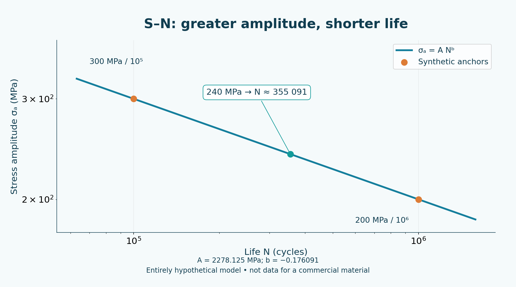
We choose two synthetic points: an amplitude of 300 MPa at 100000 cycles and 200 MPa at 1000000 cycles. We do not attribute them to A36, SAE 1045 or any tested alloy. The adopted form is σ_a = A N^b, with N used numerically in cycles; other conventions may use reversals, and their coefficients must not be mixed.
The exponent is b = log10(200/300)/log10(1000000/100000) = −0.176091259. Next, A = 300/(100000)^b = 2278.125 MPa. The relationship is a straight line in logarithmic coordinates; coefficient A is neither a material’s ultimate strength nor a value measured at a single cycle.
For an amplitude of 240 MPa, N = (240/2278.125)^(1/b) = 355091.039 cycles, approximately 355091 cycles. This is interpolation between the selected points. It does not include statistical distribution, reliability, size, finish or environment. For amplitudes outside 200–300 MPa, the same model extrapolates; the lab indicates this distinction.
| Item | Value |
|---|---|
| First anchor | 300 MPa at 100000 cycles |
| Second anchor | 200 MPa at 1000000 cycles |
| b | −0.176091259 |
| A | 2278.125 MPa |
| Selected amplitude | 240 MPa |
| Mathematical life N | 355091.039 cycles |
Notches, finish, welds and corrosion change the problem
A hole, thread, keyway or abrupt change in section may increase local stress relative to nominal stress. K_t is the theoretical elastic stress concentration for a geometry and loading condition. K_f describes a fatigue concentration effect in an appropriate approach; it is not automatically equal to K_t.
The conceptual relationship K_f = 1 + q(K_t − 1), with notch sensitivity q between zero and one, is an approximation used under relevant conditions. Material, size and geometry influence its use. Applying this factor uncritically to a weld does not replace welded-detail standards, structural-stress methods or relevant tests.
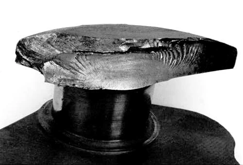
Roughness, machining marks, transition radii and corrosion may affect initiation and propagation. Residual stresses may be tensile or compressive; treatments and welding also change the microstructure. A crankshaft photograph shows a real component but does not allow K_t or K_f to be calculated or every factor in its fracture to be diagnosed.

Exercise 2: tensile mean stress on the Goodman diagram
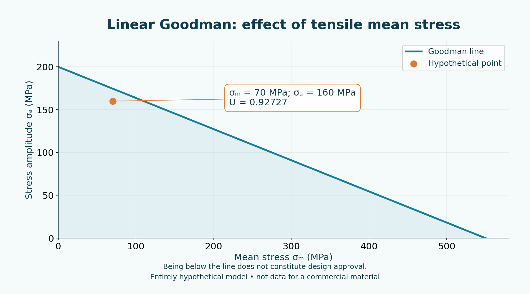
For another independent model, we adopt hypothetical references S_e = 200 MPa and S_ut = 550 MPa. S_e is the fatigue reference chosen for this Goodman exercise, not a plateau demonstrated by the preceding Basquin curve. S_ut represents hypothetical ultimate strength; yield strength is a different property.
With σ_a = 160 MPa and σ_m = 70 MPa, the linear index is U = σ_a/S_e + σ_m/S_ut = 160/200 + 70/550 = 0.9272727. The point lies below the U = 1 line. Defining a nominal factor by proportional scaling of this point gives n = 1/U = 1.078431.
This reciprocal is not a design safety factor or project approval. It does not check yielding, scatter, geometry or all failure mechanisms. The lab restricts mean stress to tensile or zero values; compressive mean stresses require appropriate treatment and context rather than extending the line as a universal promise of benefit.
NASA RP-1123 — Design of Power-Transmitting Shafts — Stuart H. Loewenthal →
| Input or result | Value |
|---|---|
| S_e / S_ut | 200 / 550 MPa |
| σ_a / σ_m | 160 / 70 MPa |
| U | 0.9272727 |
| Nominal 1/U | 1.078431 |
| Interpretation | Mathematical position below the line; no approval |
Exercise 3: Miner adds blocks, not an exact failure date
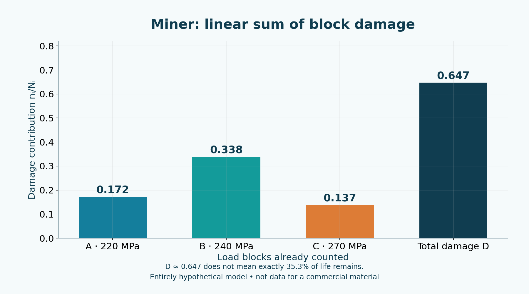
We return to the fictional Basquin curve for three already-counted blocks of fully reversed amplitude. The linear rule is D = Σ(n_i/N_i), where n_i is applied cycles and N_i the curve’s reference life at that amplitude. Each term is dimensionless; the model adds contributions without representing the physical order of application.
For 220 MPa and 100000 cycles, N = 582017.675 and n/N = 0.171816. For 240 MPa and 120000 cycles, N = 355091.039 and the contribution is 0.337942. For 270 MPa and 25000 cycles, N = 181907.667 and the contribution is 0.137432. Summing unrounded values gives D = 0.64718995.
D = 1 is a reference in the linear model, not a guarantee of rupture at that cycle. D = 0.647 does not mean exactly 35.3% of life remains. Load order, means, multiaxiality, residual stresses and environment can change actual behavior. Rainflow counting is addressed by ASTM E1049-85(2023), but this exercise does not implement the algorithm: the blocks have already been counted.
ASTM E1049-85(2023) — Cycle Counting in Fatigue Analysis →
NASA — Cumulative Axial and Torsional Fatigue in a Cobalt-Base Superalloy →
| Block | Amplitude | Cycles n | Life N | Contribution n/N |
|---|---|---|---|---|
| A | 220 MPa | 100000 | 582017.675 | 0.171816 |
| B | 240 MPa | 120000 | 355091.039 | 0.337942 |
| C | 270 MPa | 25000 | 181907.667 | 0.137432 |
| Total | — | 245000 | — | 0.647190 |
A preexisting crack: what does the Paris law describe?
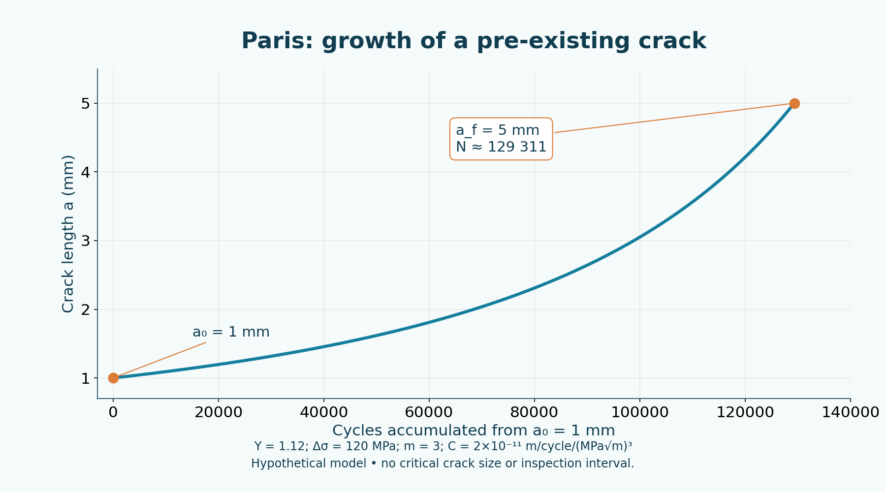
Propagation analysis begins with an existing crack. In a mode-I elastic representation, ΔK = Y Δσ √(πa) relates the stress-intensity range to stress range and length a. Y depends on geometry; ΔK has units of MPa√m when stress is in MPa and a in meters. It is neither mean stress nor directly nominal stress.
In the appropriate growth region, the Paris law is da/dN = C(ΔK)^m. Coefficients depend on material, environment, stress ratio and units. The model does not universally describe initiation, short cracks, the near-threshold region, large plastic zones or unstable fracture. ASTM E647-24 addresses growth-rate measurement; its scope is not a license to extrapolate any life.
In this entirely hypothetical advanced example, Y = 1.12 is constant, Δσ = 120 MPa, m = 3 and C = 2×10⁻¹¹ m/cycle/(MPa√m)³. We adopt a₀ = 1 mm and a_f = 5 mm, converted to 0.001 and 0.005 m. Integration gives N = 2(a₀^(−1/2) − a_f^(−1/2))/[C(YΔσ√π)³] = 129310.782 cycles.
The final 5 mm size was chosen for the exercise, not calculated as a critical crack. Assessment of K_max, fracture resistance, dimensions and actual conditions is missing. The result does not determine an inspection interval. The chart uses cycles actually elapsed, and the lab rejects a_f less than or equal to a₀ rather than displaying fictitious propagation.
Fractography: beach marks are not striations
Beach marks are macroscopic features of progressive advance that may appear on a fatigue surface. Striations are microscopic features examined, for example, by scanning electron microscopy. These are different scales and types of evidence; we should not automatically equate a mark with a cycle or assume every material shows both.
The absence of macroscopic marks does not eliminate the fatigue hypothesis. Oxidation, post-fracture rubbing, multiple origins and different mechanisms can complicate interpretation. Initiation at holes, inclusions, welds or a surface is a possibility to investigate, not a diagnosis to apply through visual similarity.
Carlos Delgado’s real fracture surface and the zone diagram serve different purposes: the photograph documents a component identified by its author; the diagram teaches a possible conceptual pattern. A reliable investigation relates fracture evidence to history, geometry, material and service conditions.
NASA RP-1291 — Fractography Handbook of Spaceflight Metals — Rebecca J. Derro →

Historical case: Aloha Airlines 243 in 1988
On April 28, 1988, Aloha Airlines Flight 243 suffered structural rupture and in-flight decompression. This case is presented as a historical integrity and maintenance study based on NTSB documentation and the FAA’s technical summary. It is not a recent accident report or proof that metal age alone explains a failure.
The NTSB attributed the probable cause to the maintenance program’s failure to detect significant disbonding and fatigue damage in a longitudinal fuselage joint. The documentation also discusses contributing factors involving oversight and evaluation, inspection scope and difficulties associated with the joints. Reducing the occurrence to a single crack or old metal would lose an essential part of the conclusion.
The FAA explains the context of fatigue damage at rivet holes, multiple cracks and joint deterioration. The lesson concerns both the physical path of damage and organizational barriers: design, instructions, execution and inspection effectiveness must work together. We do not use photographs of victims or FAA images with unlicensed third-party rights.
Damage tolerance considers the possibility of defects and their evolution in a structure, with assessments and inspections supported by relevant criteria. FAA AC 25.571-1D addresses this context for transport airplanes. It is a sector-specific reference, not a universal standard authorizing an industrial component using this lab’s numbers.
NTSB — Aloha Airlines Flight 243 — DCA88MA054 →
FAA — Aloha Airlines Flight 243: Lessons Learned →
FAA — AC 25.571-1D — Damage Tolerance and Fatigue Evaluation of Structure →
Shafts, bolts, springs and supports in our machines
A pump shaft may experience cyclic bending; an oscillating support, weld, rotor or bolted joint may receive different load histories. Preload, alignment, resonance and operating conditions need case-specific examination. These examples connect the topic to machinery without diagnosing particular equipment.
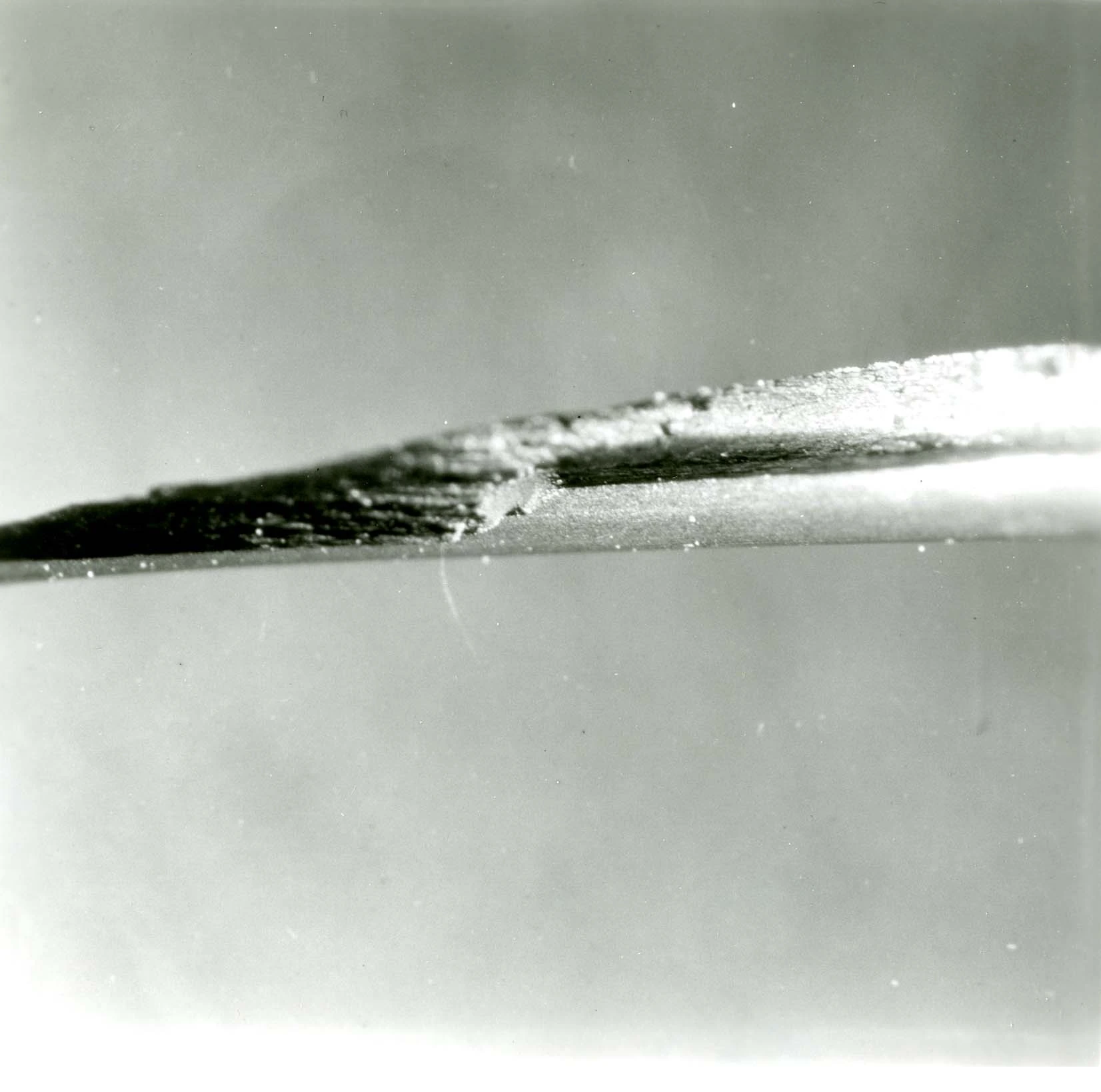
The historical spring photograph from the NIST collection documents fatigue research and observation in a real component. Like the crankshaft image, it helps visualize the phenomenon’s relevance beyond a chart. The article’s synthetic curves are not data from these components or results attributed to their materials.
Tracking hours, cycles, events, manufacturing, treatments, material and maintenance helps formulate better hypotheses. The previous article on pumps and cavitation examines another damage mechanism; recognizing a failure requires distinguishing mechanisms rather than using fatigue as a generic explanation for any broken part.
nist-spring-photo.webp — source, author and use conditions →
Investigate while preserving evidence
Safety and isolation of the hazardous condition come first. The investigation then seeks to preserve the component, its position, loading direction and service records. Grinding, welding, aggressive cleaning or discarding the surface before documentation can remove relevant evidence.
Overview and close-up photographs, drawings, material, treatments and history help guide examinations. Depending on the case, metallography, microscopy and nondestructive testing add evidence. Selection depends on material, defect type and orientation, access and sensitivity; an inspection without indications does not establish the absence of every crack.
An estimated-life result must state the model, data, assumptions and uncertainties. The chain of evidence is more valuable than a rushed conclusion based on appearance or a single formula.
FAA — Fatigue and Damage Tolerance →
Functional safety: PLC and two-hand control →
- Document the component, position, orientation and surfaces before altering evidence.
- Collect drawings, material, treatments, welds and manufacturing history.
- Relate hours, cycles, loads, transients, environment and maintenance.
- Select relevant examinations and record detection and interpretation limits.
- Test hypotheses against evidence and maintain traceability of conclusions.
Interactive lab: four questions, four models
Select S–N, Goodman, Miner or Paris. Controls let you vary amplitude, tensile mean stress, the cycles in three blocks and crack-path parameters. Equivalent tables display data without relying solely on charts. Labels and notices appear in the page’s language.
Restore each example to reproduce the calculations. In S–N, observe the interpolation or extrapolation indication. In Goodman, compare the position relative to the line without treating it as approval. In Miner, change blocks and cycles without interpreting D as an exact percentage of consumed life. In Paris, keep final length above initial length and check units.
All data are invented for learning. Calculations run in the browser without sending inputs. The standalone HTML has a PT/EN/ES selector; Python, CSV and the package with figures and credits allow reproduction. Without JavaScript, static exercises remain available, but fields do not update results.
Fatigue laboratory: synthetic data
Four independent teaching models. Local calculations; inputs are not sent to facilities or external services.
Does not establish safety, service life, compliance or inspection intervals. Do not automatically add Basquin life to Paris propagation; their questions and assumptions differ.
S–N / Basquin
- Mathematical life N (cycles)
- 355,091
- Selected amplitude (MPa)
- 240.000
Interpolation between the two synthetic anchors.
Equivalent chart table
| N (cycles) | σ_a (MPa) |
|---|---|
| 100,000 | 300.000 |
| 1,000,000 | 200.000 |
| 355,091 | 240.000 |
σ_a = A N^b; A = 2278.125 MPa; b = −0.176091259.
Fictitious curve: 300 MPa at 100000 cycles, 200 MPa at 1000000. N means cycles, not reversals. No scatter, size, finish or reliability model.
Open the standalone PT/EN/ES simulator →
Download the Python calculations →
Download synthetic data in CSV →
Load history must be understood
Nominal stress at one instant does not summarize the behavior of thousands of repetitions. S–N curves, mean-stress corrections, cumulative damage and crack growth answer different questions under different assumptions. Using a formula without identifying that question can create confidence unsupported by the data.
Vibration and resonance will be the series’ next step: how motion can amplify loads and feed this history. Fatigue is the history of loads written within the material. Designing means anticipating that history; investigating means learning to read it.
Frequently asked questions
What is metal fatigue, and why does it occur below yield strength?
It is progressive damage associated with cyclic loading. Maximum nominal stress below static yield strength does not demonstrate the absence of local concentration, microscopic deformation or defect growth. Geometry, surface, microstructure, residual stresses and environment influence the process. The number and form of repetitions also matter. An isolated static check therefore does not establish fatigue life.
What does an S–N curve mean?
It relates a measure of cyclic stress to cycles until a failure criterion under defined conditions. The quantity represented by S, stress ratio, test type and scatter must be known. This article’s fictional curve uses amplitude and two chosen points; it allows Basquin to be studied but does not characterize a commercial steel or replace experimental component data.
What is the difference between fatigue strength and fatigue limit?
Fatigue strength is associated with a life, such as N cycles, and the conditions used. Fatigue limit describes a plateau under relevant conditions when that behavior is observed. Not every metal shows a defined horizontal limit over the studied interval. The synthetic Basquin curve should not be extrapolated to conclude that lower stresses provide infinite life; model validity and experimental context must be examined.
How do mean stress and amplitude change the analysis?
Amplitude describes half the range between extremes; mean stress indicates the level around which the cycle varies. Histories with the same amplitude and different means can respond differently. Linear Goodman is a simplified correction used here with tensile mean stress and hypothetical references. Its index and nominal reciprocal neither check all mechanisms nor approve a design; compressive means require an appropriate approach.
How can signs of fatigue be identified in a real fracture?
Examine the surface together with loading, geometry, material and history. Beach marks, when present, are macroscopic; striations are microscopic and should not be confused with them. Absence of macroscopic marks does not rule out fatigue. Oxidation, rubbing and multiple origins can alter evidence. Photography helps document and frame questions, but a conclusion may require fractography, metallography and other evidence.
What is Miner’s rule, and what are its limits?
It adds fractions n_i/N_i from load blocks, producing dimensionless linear damage D. In this article, blocks are already counted and their lives come from a fictional curve. D = 1 is a mathematical reference, not a guarantee of exact failure, and D below one does not give the precise percentage of life remaining. Sequence, mean stresses, scatter, environment and other effects limit this simplification.
What is the Paris law used for?
It represents growth of an existing crack in an appropriate propagation region using da/dN = C(ΔK)^m. Coefficients, geometry, units and conditions must be defined. It does not universally cover initiation, short cracks, threshold or unstable rupture. The 1-to-5 mm example is entirely hypothetical; its final length is not critical, and calculated cycles do not establish an inspection interval.
How does nondestructive testing contribute to integrity?
It can reveal indications and support monitoring and investigation without destroying the component, depending on the method and defect. Selection considers material, orientation, size, access and sensitivity. Results must be interpreted with detection limits and relevant criteria; no indication does not prove the absence of any crack. Integrity also depends on design, manufacturing, loads, maintenance and traceability rather than a single inspection.
References
- ASTM E466-21 — Force Controlled Constant Amplitude Axial Fatigue TestsASTM International
- ASTM E647-24 — Measurement of Fatigue Crack Growth RatesASTM International
- ASTM E1049-85(2023) — Cycle Counting in Fatigue AnalysisASTM International
- NASA RP-1123 — Design of Power-Transmitting Shafts — Stuart H. LoewenthalNASA
- NASA RP-1291 — Fractography Handbook of Spaceflight Metals — Rebecca J. DerroNASA
- NASA — Cumulative Axial and Torsional Fatigue in a Cobalt-Base SuperalloyNASA
- NTSB — Aloha Airlines Flight 243 — DCA88MA054NTSB
- FAA — Aloha Airlines Flight 243: Lessons LearnedFAA
- FAA — AC 25.571-1D — Damage Tolerance and Fatigue Evaluation of StructureFAA
- FAA — Fatigue and Damage ToleranceFAA
- fracture-photo.webp — photo provenanceReal macro photograph of fatigue fracture in steel, as described by its author. Photo: Carlos Delgado / Wikimedia Commons, CC BY-SA 4.0. Resized and converted to WebP; no new annotations.
- crankshaft-photo.webp — photo provenanceFractured crankshaft surface, from the file identified as Crankshaft fatigue. Photo: Peterlewis / Wikimedia Commons, CC BY-SA 3.0. Converted to WebP; original 500 × 340 resolution retained.
- nist-spring-photo.webp — photo provenanceSpring-wire section with a fatigue crack from a historical NBS study. National Institute of Standards and Technology Digital Collections, Gaithersburg, MD 20899. Converted to WebP; no new annotations.