
Understand metal creep, rupture curves and Larson–Miller, with worked examples explaining hot piping, time-dependent deformation and limits of life prediction.
When time becomes part of the load
How can a steel tube keep deforming for thousands of hours and eventually fail without an obvious increase in load? In a steam line, a superheater or a turbine, creep may be part of the answer: time-dependent deformation promoted by temperature and governed by stress and the material's evolving microstructure.
A component may survive startup yet fail to withstand the conditions imposed over years. Comparing the applied stress with room-temperature yield strength introduces the issue, but cannot settle a hot-service assessment. Properties at operating temperature, time-dependent design criteria and the actual operating history also belong in the engineering question from the beginning.
This review connects mechanisms, tests and worked examples to explain that distinction. The numerical models and their graphs use synthetic data, unrelated to a commercial steel grade.
Homologous temperature: start with Kelvin
Homologous temperature is T/Tm, using service temperature T and a melting reference Tm on the same absolute scale, Kelvin. Dividing two Celsius readings is incorrect. For example, 550 °C equals 823.15 K. This conversion is part of the physical definition rather than a cosmetic choice about which unit appears beside a number.
Ranges such as 0.3–0.4 Tm are useful orientation when discussing creep in metals. They do not provide a universal switch separating creep-free service from damaging creep. Alloy, stress, duration, dominant mechanisms and measurement sensitivity change the response. Alloys also melt over a range, so the selected reference, such as the solidus, must be identified.
For an operating component, the relevant value is the local metal temperature, rather than only the nominal steam or gas reading. Deposits, flow distribution, insulation and cooling conditions can create important differences. A local hot spot may accumulate damage differently from the rest of a part while the overall operating indicators still appear stable.
Reading the three stages of a creep curve
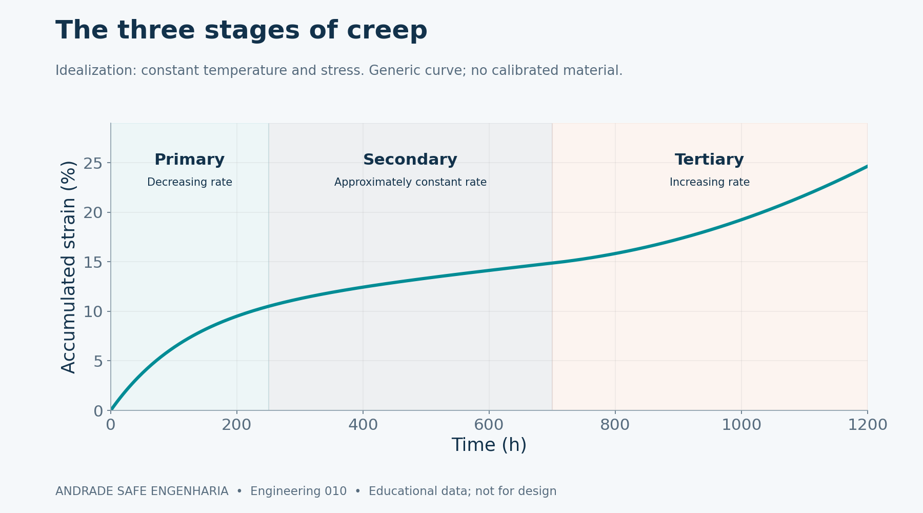
A creep curve records strain against time under defined test conditions. Following the instantaneous loading response, primary creep has a decreasing strain rate: deformation continues, but the curve becomes less steep. Strain hardening and recovery processes contribute to this evolution according to the combination of material condition, applied stress and temperature maintained during the test.
During secondary creep, the rate is approximately constant over part of the test. This region, often discussed through the minimum creep rate, supports comparison and modelling. It does not mean that the microstructure has stopped changing or that service can continue indefinitely. A small slope accumulated over many hours can still produce significant deformation in a component.
Tertiary creep involves acceleration and may include section reduction, cavities, cracking and microstructural changes. Its form depends on the material and the test. The illustration here is schematic: it supplies no allowable strain, operating alarm threshold or rupture prediction for an actual tube. Not every experimental curve displays three equally distinct regions, particularly over a limited observation period.
| Stage | Rate trend | Interpretation |
|---|---|---|
| Primary | Decreasing | Strain continues; slope falls |
| Secondary | Approximately constant | Useful region for minimum rate |
| Tertiary | Increasing | Acceleration; material-dependent mechanisms |
What changes inside the metal
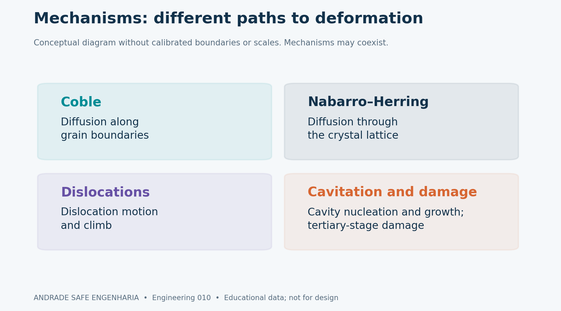
In Nabarro–Herring diffusional creep, atoms move through the crystal lattice. The idealized formulation gives an inverse-square dependence of strain rate on grain size, d⁻². In Coble creep, diffusion along grain boundaries becomes important, with an idealized d⁻³ dependence. These relationships describe particular conditions rather than every steel exposed to elevated temperature in service.
Dislocation creep involves the motion of crystalline defects, including climb and recovery processes that allow deformation to develop over time. The rate can be strongly stress-sensitive, often represented using a power law. Precipitates, solid solution strengthening and microstructural stability affect resistance. Nominal composition and temperature alone therefore do not provide a complete description of the response.
Grain-boundary cavities may develop and coalesce as damage progresses, but they are not the sole explanation for every creep fracture. Multiaxial loading, the environment, welds and metallurgical evolution also matter.
Creep tests and tests to rupture
ASTM E139-24 addresses creep, creep-rupture and stress-rupture tests of metallic materials. Its public scope describes determining deformation with time and time to fracture under constant tensile force and constant temperature. This summary relies on the available official abstract; it does not reproduce detailed procedures or requirements from the complete standard, which must be consulted for its intended application.
When deformation is the focus, tracking elongation and time produces the curve and quantities such as minimum creep rate. In a rupture test, time to fracture is a central response, together with the conditions and relevant specimen information. Comparisons should account for geometry, measurement, temperature control, metallurgical condition and scatter, rather than comparing the reported hours in isolation.
Constant force does not mean constant true stress. If the load-bearing section decreases while force remains unchanged, true stress increases. Nominal stress may still be reported using the initial area, but that convention does not remove local evolution. The distinction helps explain tertiary acceleration and prevents laboratory curves from being interpreted as perfectly unchanging stress states throughout a test.
ASTM E139-24 — Creep, Creep-Rupture, and Stress-Rupture Tests →
| Test / control | Observation | Caution |
|---|---|---|
| Creep | Strain versus time | Control and measurement matter |
| Rupture | Time to fracture | Scatter and metallurgical condition |
| Constant force | Maintained load | True stress may increase |
Rupture curves: time is not a standalone property
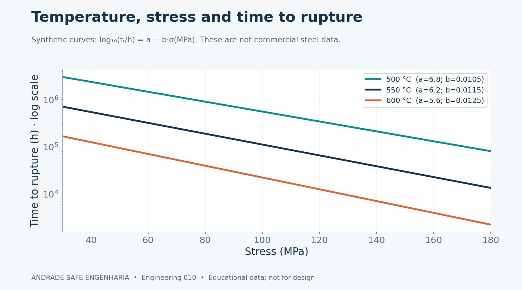
A family of stress-versus-rupture-time curves allows comparison of results obtained at defined temperatures. Increasing stress or temperature generally reduces rupture time within the usual ranges being considered. Time is often plotted logarithmically to cover orders of magnitude. Equal distances on that axis represent equal ratios, rather than equal additions of hours to the test duration.
For teaching purposes only, this article uses log10(tr/h) = a − b·(σ/MPa). Here tr is rupture time in hours, σ is stress in MPa, and a and b are synthetic coefficients assigned to each temperature curve. They do not come from manufacturer tables, an ASME allowable-stress source or experiments on an identified steel grade.
A fitted straight line does not guarantee safe extrapolation. In real materials, mechanism changes, aging, welding and experimental scatter may alter the relationship between stress and duration. The further a proposed application lies outside the tested range, the more carefully its physical and statistical justification must be examined.
Larson–Miller: correlation with a defined convention
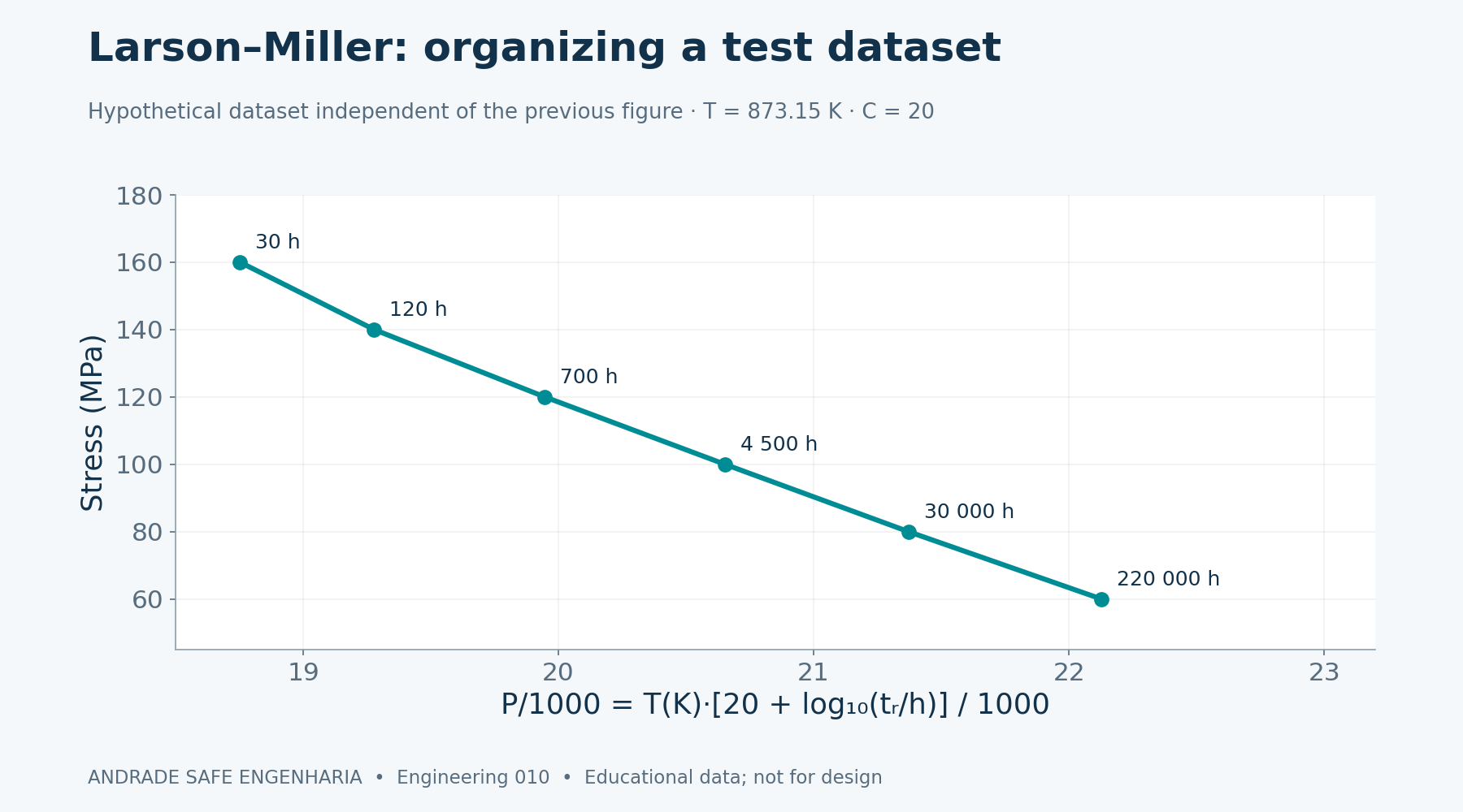
The Larson–Miller parameter combines absolute temperature and rupture time: P = T·[C + log10(tr/h)]. Temperature T is in Kelvin; writing tr/h explicitly states that the logarithm uses the numerical time in hours. C is a correlation constant that must be defined and fitted for the dataset and the convention used to report its results.
Here C = 20 is a teaching assumption, rather than a universal constant for steel. Dividing P by 1,000 simply makes the graph scale more convenient. Changing the time unit without adapting the convention for C changes the result; using Celsius instead of Kelvin also undermines the interpretation.
The Larson–Miller figure uses a separate synthetic dataset: at 600 °C, stresses of 160, 140, 120, 100, 80 and 60 MPa correspond to 30, 120, 700, 4,500, 30,000 and 220,000 h. This dataset is independent of the preceding rupture lines. It does not represent the same alloy and must not be combined with those lines to invent a certified master curve.
Worked example 1: check the tube geometry first
Consider internal pressure p = 10 MPa, outside diameter Do = 50 mm and wall thickness t = 5 mm. The outside radius is ro = 25 mm and the inside radius is ri = 20 mm. The simplified expression p·Do/(2t) gives 50 MPa, but t/ri = 0.25: treating this wall as thin is unjustified for this example.
For an idealized elastic cylinder with no external pressure, Lamé's solution gives the inner-wall hoop stress: σθ(ri) = p·(ri² + ro²)/(ro² − ri²). Substituting consistent units gives 10·(400 + 625)/(625 − 400) = 45.5556 MPa. This is the elastic circumferential stress component at the specified location, under the assumptions of that cylinder solution.
Even the corrected geometry calculation does not design a hot pipe. Pressure creates other stress components; end conditions, restraints, weight, thermal expansion, welds and thickness loss may all require consideration. Lamé's elastic result alone describes neither creep redistribution nor multiaxial creep life. The first lesson is to check assumptions before trusting an apparently persuasive numerical answer.
| Quantity | Value | Limit |
|---|---|---|
| p; Do; t | 10 MPa; 50 mm; 5 mm | Hypothetical geometry |
| ri; ro; t/ri | 20 mm; 25 mm; 0.25 | Thin-wall assumption unjustified |
| pDo/(2t) | 50 MPa | Inadequate approximation here |
| Lamé: σθ(ri) | 45.5556 MPa | Inner elastic component; no creep assessment |
Worked example 2: temperature rises at an assumed fixed stress
Now choose σ = 50 MPa as an independent teaching assumption, without assigning it to the preceding pipe. For the synthetic 550 °C curve, a = 6.2 and b = 0.0115; at 600 °C, a = 5.6 and b = 0.0125. Calculate the logarithm first and then raise ten to that power, retaining the stated MPa-and-hours convention.
At 550 °C, log10(tr/h) = 6.2 − 0.0115·50 = 5.625, giving approximately 421,696.50 h. At 600 °C, the exponent is 5.6 − 0.0125·50 = 4.975, giving 94,406.09 h. Within these two invented curves, the second duration is about 22.4% of the first, representing a reduction of approximately 77.6% at the same assumed stress.
The ratio between the durations is about 4.47. It illustrates thermal sensitivity in this particular example, rather than a rule that every 50 °C increase divides life by that factor. These durations are not an authorized service life, remaining life or inspection interval. They must not be turned into a recommendation to keep a specific operating component in service.
| Synthetic curve | Exponent log10(tr/h) | Time |
|---|---|---|
| 550 °C; a = 6.2; b = 0.0115 | 5.625 | 421,696.50 h |
| 600 °C; a = 5.6; b = 0.0125 | 4.975 | 94,406.09 h |
| Comparison | Ratio ≈ 4.47 | Reduction ≈ 77.6% |
Worked example 3: a normalized Norton–Bailey expression
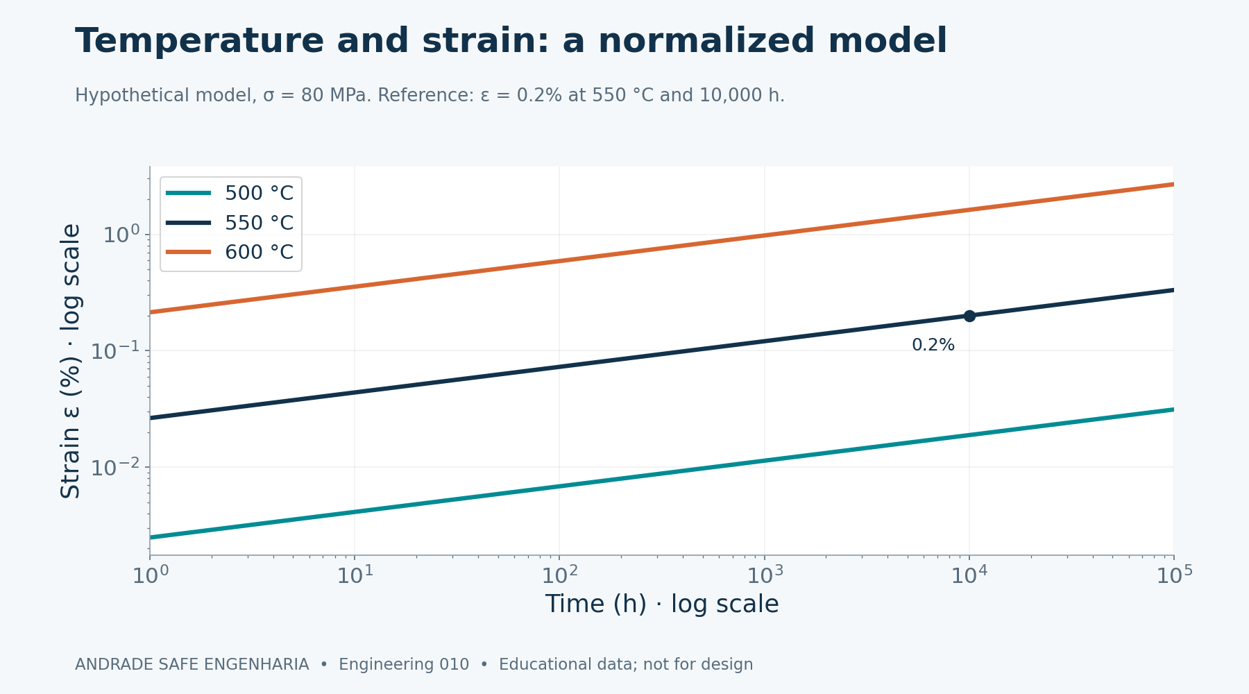
To explore trends without ambiguous dimensional coefficients, use ε = 0.002·(σ/80 MPa)^5.2·(t/10,000 h)^0.22·exp{−(250,000/8.314)·[1/T − 1/823.15]}. Strain ε is dimensionless and T is in Kelvin. The assumed activation energy is 250,000 J/mol and R = 8.314 J/(mol·K). Every numerical model coefficient is hypothetical, rather than certified data for a commercial steel.
At the reference condition, σ = 80 MPa, t = 10,000 h and T = 823.15 K, the normalized factors equal one, giving ε = 0.002, or 0.2%. The stress exponent 5.2 makes the result strongly load-sensitive. The exponential term increases with temperature. Directly entering Celsius or replacing MPa with Pa without changing the formula destroys numerical consistency.
Because the time exponent is 0.22, this expression produces a decreasing rate for positive time. It models neither a constant-rate secondary region nor tertiary acceleration or rupture. The laboratory does not declare failure after an arbitrary strain percentage is crossed. Conceptually comparing it with the static rupture curves helps distinguish questions and models; it does not combine them into a prognostic tool.
Where creep meets field engineering
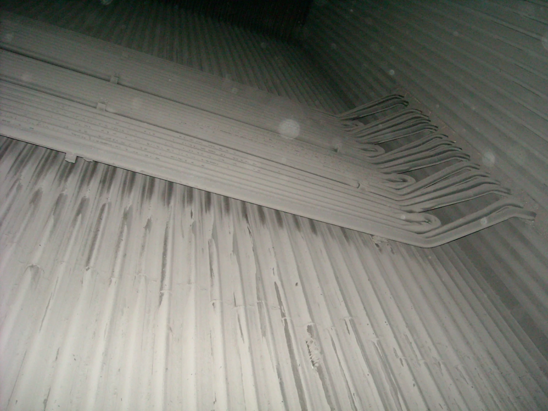
Superheater and reheater tubes combine pressure, prolonged thermal exposure and possible differences between fluid and metal temperatures. Steam lines also experience support loads, thermal expansion and restraint. A useful assessment connects the likely mechanism with stress distribution and local temperature. Treating every hot component under the same simplified strength rule overlooks the conditions that actually control its response.
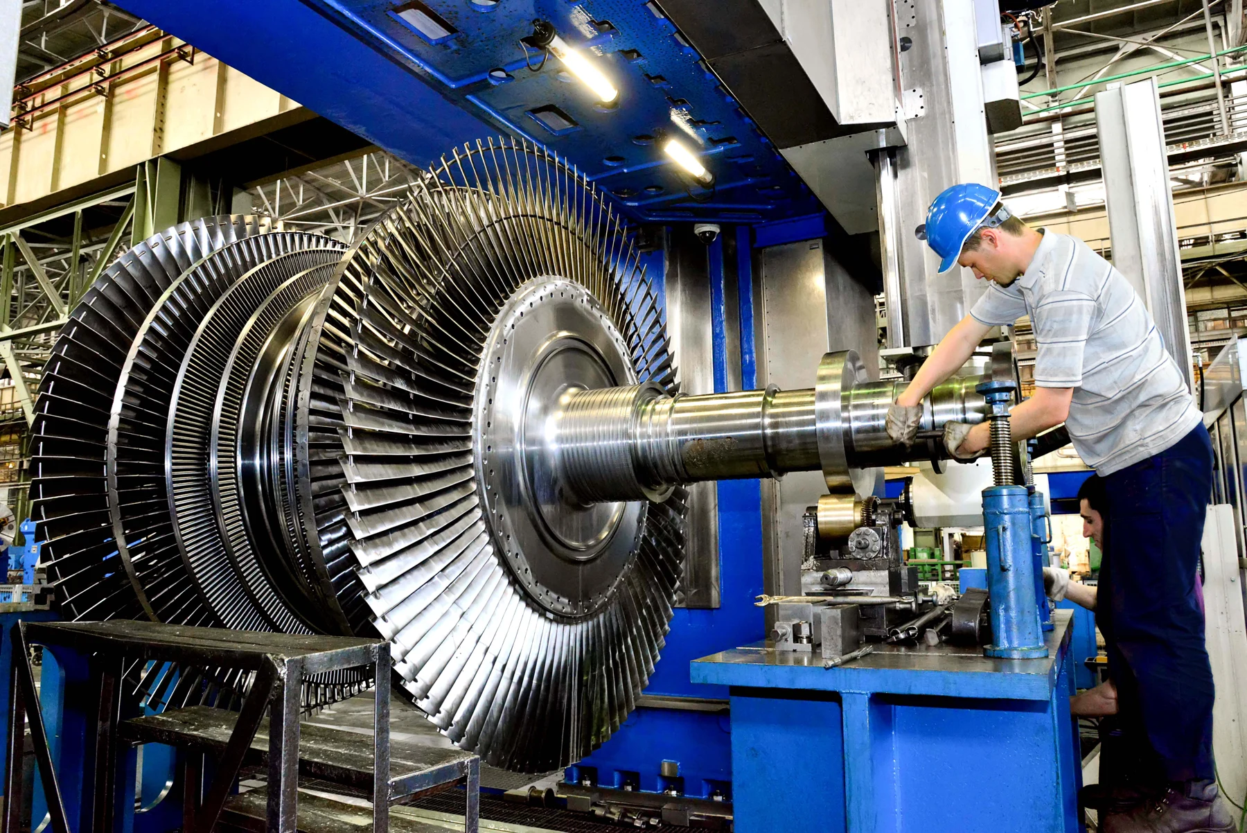
Hot turbine parts, rotors and casings can have markedly different service conditions. Material, cooling, gradients and operating cycles determine which mechanisms deserve priority. Selecting a creep-resistant alloy involves microstructural stability and environment as well as instantaneous strength. There is no single operating-temperature limit that can be assigned generically to every steel grade or every turbine component without further qualification.
Creep can interact with thermal and mechanical fatigue, oxidation and high-temperature corrosion. Each shutdown and startup adds stress and temperature variations to the history. Distinguishing sustained loading from cyclic loading is conceptually useful, but actual equipment may require assessment of creep-fatigue interaction and environmental damage together. An isolated model cannot automatically account for those concurrent and sometimes interacting processes.
Boiler tube failure mechanisms →
Signs of damage: observations before conclusions
Bulging, ovality and progressive permanent deformation warrant investigation, particularly after prolonged high-temperature exposure. Thickness loss may increase stress and alter geometry, while deposits may change thermal conditions. None of these signs independently identifies the cause or quantifies remaining life. Comparing repeatable measurements over time helps reveal progression and gives the observations a more useful engineering context.
Metallographic replicas can reveal features of a prepared surface and support investigation of cavitation, depending on the material and technique. Metallography, hardness, nondestructive testing, dimensional checks and operating records answer different questions. Failure to find cavities in a small examined area does not demonstrate the absence of damage throughout the volume, across welds or in regions with different temperatures.
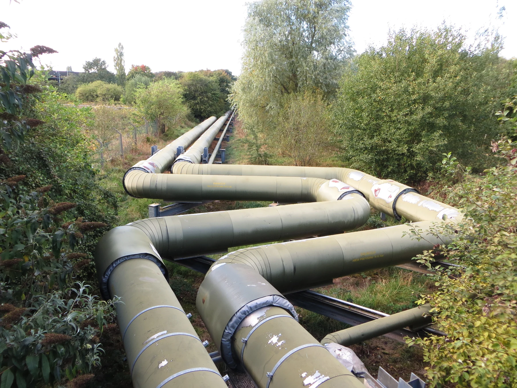
An investigation should record location, method, repeatability, thickness, surface condition and available history. A sound diagnosis connects evidence with plausible mechanisms while recognizing limitations of access and representativeness. Equipment photographs illustrate applications; they do not justify claiming creep damage in the pictured parts unless the image source actually documents that condition. Appearance alone cannot establish a metallurgical diagnosis.
Why remaining life requires more than a calculator
Remaining life depends on the installed material, manufacturing condition, welds, current geometry and pressure-temperature history. Operating hours without context may hide overheating, transients and service changes. Alloy identification and traceability become particularly important when published rupture data are proposed to represent a specific component. The choice of a familiar material name cannot resolve uncertainty about the actual installed condition.
An assessment method must state its criteria, properties, uncertainties and domain of validity. Long extrapolations, experimental scatter and multiaxial stress do not disappear when a well-known equation is selected. Accumulated-damage assumptions also need justification: adding simplified life fractions does not turn hypothetical inputs into adequate evidence for releasing equipment or scheduling its next inspection without the necessary engineering basis.
In practice, integrity assessment joins documentation, inspection, analysis and responsible technical decisions. The examples here help readers formulate better questions; they replace neither material selection nor calculations under applicable criteria or a fitness-for-service assessment of actual equipment.
Educational laboratory and study downloads
The downloadable laboratory varies stress, temperature and time in the normalized strain expression. Start at the reference of 550 °C, 80 MPa and 10,000 h, changing one variable at a time. Controls cover 450–600 °C, 30–100 MPa and 1–100,000 h; these are teaching limits rather than a validated material range.
The scenario CSV and Python model make inputs and outputs auditable. Check units before comparing results: dimensionless strain is not percentage strain, Kelvin is not Celsius, and exposure duration is not automatically time to fracture. The HTML displays strain, its time derivative, the thermal factor and the ratio of calculated strain to the 0.2% reference. Rupture curves remain static in the article and kit files. A warning above 5% strain only flags large deformation in the exercise; it signifies neither rupture nor operational acceptance or rejection.
The HTML is educational; it represents neither a commercial material nor actual equipment or operational authorization. Check photo credits for authorship and context, and institutional references for further study.
Open the educational laboratory PT/EN/ES →
Download synthetic CSV scenarios →
Withstanding a load also means withstanding it long enough
Creep connects atomic movement, microstructure, stress and duration. Understanding the stages helps interpret tests; recognizing geometry avoids using an approximation outside its assumptions; separating correlation from actual data prevents an elegant curve from becoming false certainty about life. Following that path makes theory useful when observing hot components and deciding which evidence needs closer examination.
In creep, temperature gives atoms mobility and time becomes part of the demand on the material. For boilers, piping and turbines, the question must include how long, at what temperature and under which conditions the part must resist. A defensible engineering answer starts with those conditions and continues through evidence, rather than ending with the first calculation.
Frequently asked questions
What is metal creep?
Creep is time-dependent deformation under stress. Its service relevance depends on temperature, duration, material and microstructure. In hot components it can control deformation and rupture without an increase in external load.
At what temperature does creep become important?
There is no universal temperature. T/Tm in Kelvin provides orientation; ranges such as 0.3–0.4 Tm do not replace alloy properties, stress, duration and the actual local metal temperature.
What are the three creep stages?
Primary creep has a decreasing rate. Secondary creep has an approximately constant rate over part of a test. Tertiary creep accelerates. Their visibility and extent depend on material and test conditions.
Does constant load mean constant stress?
Not necessarily. Under constant force, decreasing area raises true stress. Nominal stress based on the initial area does not describe that local evolution.
What is creep rupture?
It is fracture after exposure to stress and temperature for a period of time. It differs from accumulated deformation, which can be measured before fracture and does not alone establish an allowable service life.
How does the Larson–Miller parameter work?
It correlates absolute temperature with logarithmic rupture time. Here P = T[C + log10(tr/h)] uses Kelvin and a hypothetical C = 20. The fitted constant and unit convention must remain consistent.
Is the example pipe thin-walled?
The adopted geometry gives t/ri = 0.25, so that approximation is unjustified. Its 50 MPa is not a validated stress. Lamé gives 45.5556 MPa inner-wall elastic hoop stress without assessing creep or designing hot service.
Does Norton–Bailey predict laboratory rupture?
No. The normalized expression calculates hypothetical strain with a decreasing rate. It represents neither secondary nor tertiary creep and sets no strain threshold for declaring failure.
Does a replica without cavities prove absence of damage?
No. A replica represents a prepared surface and the examined area. Local absence of cavities cannot demonstrate integrity throughout the volume, in welds or in regions with different thermal exposure.
Can these results establish remaining life?
No. Coefficients are synthetic and the datasets are independent. Remaining-life assessment needs identified material, geometry, history, inspection, representative properties and a suitable technical method for the component.
References
- ASTM E139-24 — Creep, Creep-Rupture, and Stress-Rupture TestsASTM International
- Creep Deformation of Metals — DoITPoMS, Section 4University of Cambridge / DoITPoMS, hosted by Engineering LibreTexts
- What is the Larson-Miller parameter?TWI
- Early Stage Creep in CSEF Steels — report abstractTWI
- Thick Walled CylindersUniversity of Washington
- Boiler tube failure mechanismsNational Board / Babcock & Wilcox
- DoITPoMS — IntroductionUniversity of Cambridge / DoITPoMS, hosted by Engineering LibreTexts
- DoITPoMS — Creep MechanismsUniversity of Cambridge / DoITPoMS, hosted by Engineering LibreTexts
- Wikimedia Commons — Surchauffeur.JPGMeblue
- CC BY-SA 3.0Creative Commons
- Wikimedia Commons — Steam pipes (30222562375).jpgAlex Liivet
- CC0 1.0Creative Commons
- Wikimedia Commons — Steam turbine rotor.jpgElena Venediktova
- CC BY-SA 2.0Creative Commons